Examples of time-series forecasting with Python

Examples of time-series forecasting with Python#

Building on the excellent (and freely available!) Forecasting: Principles and Practice (3rd edition) by Hyndman and Athanasopoulos, this notebooks presents a number of examples using the following Python libraries:
- statsmodels.tsa as the basis for time-series analysis
- pmdarima which wraps statsmodels into a convenient auto.arima function like in R
- TO DO: sktime as the new, unified framework for machine learning in Python
Use Altair for plotting, as an example how to use this library throughout your workflow

import altair as alt
import numpy as np
import pandas as pd
import rdata
import requests


# https://altair-viz.github.io/user_guide/faq.html#local-filesystem
# alt.data_transformers.enable("json")


def read_rda(url):
    """Reads .rda file from URL and returns dict with values.
    
    """
    r = requests.get(url)
    parsed = rdata.parser.parse_data(r.content)
    return rdata.conversion.convert(parsed)

EDA with an interactive dashboard#

Bike sharing dataset#

As an example, we will explore the bike sharing dataset, taken from the UCI Machine Learning Repository

Data Set Information#

Bike sharing systems are new generation of traditional bike rentals where whole process from membership, rental and return back has become automatic. Through these systems, user is able to easily rent a bike from a particular position and return back at another position. Currently, there are about over 500 bike-sharing programs around the world which is composed of over 500 thousands bicycles. Today, there exists great interest in these systems due to their important role in traffic, environmental and health issues.

Apart from interesting real world applications of bike sharing systems, the characteristics of data being generated by these systems make them attractive for the research. Opposed to other transport services such as bus or subway, the duration of travel, departure and arrival position is explicitly recorded in these systems. This feature turns bike sharing system into a virtual sensor network that can be used for sensing mobility in the city. Hence, it is expected that most of important events in the city could be detected via monitoring these data.

Attribute Information#

Both hour.csv and day.csv have the following fields, except hr which is not available in day.csv

instant: record index
dteday : date
season : season (1:winter, 2:spring, 3:summer, 4:fall)
yr : year (0: 2011, 1:2012)
mnth : month ( 1 to 12)
hr : hour (0 to 23)
holiday : weather day is holiday or not (extracted from [Web Link])
weekday : day of the week
workingday : if day is neither weekend nor holiday is 1, otherwise is 0.

weathersit :
- 1: Clear, Few clouds, Partly cloudy, Partly cloudy
- 2: Mist + Cloudy, Mist + Broken clouds, Mist + Few clouds, Mist
- 3: Light Snow, Light Rain + Thunderstorm + Scattered clouds, Light Rain + Scattered clouds
- 4: Heavy Rain + Ice Pallets + Thunderstorm + Mist, Snow + Fog

temp : Normalized temperature in Celsius. The values are derived via (t-t_min)/(t_max-t_min), t_min=-8, t_max=+39 (only in hourly scale)
atemp: Normalized feeling temperature in Celsius. The values are derived via (t-t_min)/(t_max-t_min), t_min=-16, t_max=+50 (only in hourly scale)
hum: Normalized humidity. The values are divided to 100 (max)
windspeed: Normalized wind speed. The values are divided to 67 (max)
casual: count of casual users
registered: count of registered users
cnt: count of total rental bikes including both casual and registered

def parse_date_hour(date, hour):
    """Construct datetime for index of hourly data."""
    return pd.to_datetime(" ".join([date, str(hour).zfill(2)]), format="%Y-%m-%d %H")


daily = pd.read_csv("./bike-sharing/bike-sharing-daily-processed.csv", parse_dates=["dteday"]).drop(
    columns=["instant", "Unnamed: 0"]
)
hourly = pd.read_csv("./bike-sharing/hour.csv").drop(columns=["instant"])
hourly.index = pd.DatetimeIndex(
    hourly.apply(lambda row: parse_date_hour(row.dteday, row.hr), axis=1),
    name="timestamp",
)
daily.head()

	dteday	season	yr	mnth	holiday	weekday	workingday	weathersit	temp	atemp	hum	windspeed	casual	registered	cnt	days_since_2011
0	2011-01-01	SPRING	2011	1	NO HOLIDAY	SAT	NO WORKING DAY	MISTY	8.175849	28.363250	80.5833	10.749882	331	654	985	0
1	2011-01-02	SPRING	2011	1	NO HOLIDAY	SUN	NO WORKING DAY	MISTY	9.083466	28.027126	69.6087	16.652113	131	670	801	1
2	2011-01-03	SPRING	2011	1	NO HOLIDAY	MON	WORKING DAY	GOOD	1.229108	22.439770	43.7273	16.636703	120	1229	1349	2
3	2011-01-04	SPRING	2011	1	NO HOLIDAY	TUE	WORKING DAY	GOOD	1.400000	23.212148	59.0435	10.739832	108	1454	1562	3
4	2011-01-05	SPRING	2011	1	NO HOLIDAY	WED	WORKING DAY	GOOD	2.666979	23.795180	43.6957	12.522300	82	1518	1600	4

brush = alt.selection(type='interval', encodings=['x'])

base = (alt
 .Chart(daily)
 .mark_line()
 .encode(x='dteday', y='cnt')
 .properties(width=700, height=200)
 )

overview = base.properties(height=50).add_selection(brush)
detail = base.encode(alt.X('dteday:T', scale=alt.Scale(domain=brush)))

/opt/hostedtoolcache/Python/3.8.18/x64/lib/python3.8/site-packages/altair/utils/deprecation.py:65: AltairDeprecationWarning: 'selection' is deprecated.
   Use 'selection_point()' or 'selection_interval()' instead; these functions also include more helpful docstrings.
  warnings.warn(message, AltairDeprecationWarning, stacklevel=1)
/opt/hostedtoolcache/Python/3.8.18/x64/lib/python3.8/site-packages/altair/utils/deprecation.py:65: AltairDeprecationWarning: 'add_selection' is deprecated. Use 'add_params' instead.
  warnings.warn(message, AltairDeprecationWarning, stacklevel=1)

detail & overview

monthly = daily.groupby(['yr', 'mnth'], as_index=False)['cnt'].sum('cnt')
monthly['yr_mnth'] = monthly.apply(lambda df: '-'.join([str(df.yr), str(df.mnth).zfill(2)]), axis=1)

def simple_ts_plot(df, x='yr_mnth', y='cnt', width=700, height=200):
    return alt.Chart(df).mark_line().encode(x=x, y=y).properties(width=width)

simple_ts_plot(monthly)

Decomposition#

Simple decomposition (`statsmodels`)#

from statsmodels.tsa.seasonal import seasonal_decompose, STL

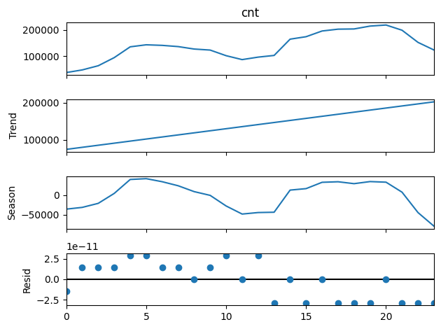
simple_decomposition = seasonal_decompose(monthly.cnt, period=12)
simple_decomposition.plot();

../_images/ab85b65e9a410a746c0245bec7eaf382e46c4d262a2ff1ec1a7d4a45ccd67404.png

STL decomposition (`statsmodels`)#

stl = STL(monthly.cnt, period=12).fit()
stl.plot();

../_images/05930c00f574e085dbcf90e165fa527d4e3a80e7fdbc9829722467f5744d6232.png

Let’s make those plots better looking with Altair.

_ts = {}
for result in ['observed', 'trend', 'seasonal', 'resid']:
    df = pd.DataFrame({'yr_mnth': monthly.yr_mnth, result: getattr(stl, result)})
    _ts[result] = simple_ts_plot(df, x='yr_mnth', y=result, height=50)


alt.vconcat(*_ts.values()).resolve_scale(x='shared')

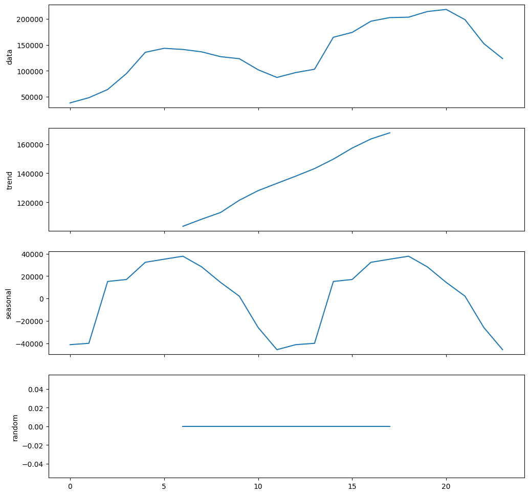
Seasonal decomposition (`pmdarima`)#

Same result as statsmodels seasonal_decompose.

from pmdarima import arima, utils

# note pmdarima expects nd.array as input
arima_decomp = arima.decompose(monthly.cnt.values, type_='additive', m=12)
utils.decomposed_plot(arima_decomp, figure_kwargs={'figsize': (12,12)})

../_images/0c30045b6c5bae759d1c1bc1bafc0a66fdb9a30a97b745d013fc8a73da6029b5.png

Forecasting with ETS#

We will reproduce the analysis from FPP2 section 7.7 in Python. following the example from the statsmodels documentation.

Get data: international visitor nights in Australia#

# read data and set proper DateRangeIndex in pandas
austourists_url = "https://github.com/robjhyndman/fpp2-package/blob/master/data/austourists.rda?raw=true" 
austourists_data = read_rda(austourists_url)
austourists = pd.DataFrame(austourists_data).set_index(
    pd.period_range(start="1999Q1", end="2015Q4", freq="Q")
)
austourists.head()

	austourists
1999Q1	30.052513
1999Q2	19.148496
1999Q3	25.317692
1999Q4	27.591437
2000Q1	32.076456

Forecast ETS(M, A, M) model#

Note: use exponential_smoothing.ETSModel and notholtwinters.ExponentialSmoothing

from statsmodels.tsa.exponential_smoothing.ets import ETSModel


aust_ets = ETSModel(
    austourists.austourists.rename('observed'), # NB: only take 1D array or pd.Series
    error="mul",
    trend="add",
    seasonal="mul",
    damped_trend=True,
    seasonal_periods=4
).fit(maxiter=10000)

print(aust_ets.summary())

RUNNING THE L-BFGS-B CODE

           * * *

Machine precision = 2.220D-16
 N =            9     M =           10

At X0         1 variables are exactly at the bounds

At iterate    0    f=  3.47328D+00    |proj g|=  1.98628D+00

At iterate    1    f=  3.14211D+00    |proj g|=  2.46124D+00

At iterate    2    f=  2.58862D+00    |proj g|=  5.91331D-01

At iterate    3    f=  2.46717D+00    |proj g|=  4.83241D-01

At iterate    4    f=  2.43892D+00    |proj g|=  6.51827D-01

At iterate    5    f=  2.37965D+00    |proj g|=  3.91487D-01

At iterate    6    f=  2.34624D+00    |proj g|=  3.02613D-01

At iterate    7    f=  2.32328D+00    |proj g|=  3.61819D-01

At iterate    8    f=  2.30622D+00    |proj g|=  1.60187D-01

At iterate    9    f=  2.29895D+00    |proj g|=  1.69179D-01

At iterate   10    f=  2.28998D+00    |proj g|=  1.79909D-01

At iterate   11    f=  2.28880D+00    |proj g|=  3.09700D-01

At iterate   12    f=  2.28586D+00    |proj g|=  8.68166D-02

At iterate   13    f=  2.28339D+00    |proj g|=  8.95314D-02

At iterate   14    f=  2.27444D+00    |proj g|=  5.47130D-01

At iterate   15    f=  2.26329D+00    |proj g|=  8.34884D-01

At iterate   16    f=  2.26104D+00    |proj g|=  7.65831D-01

At iterate   17    f=  2.26051D+00    |proj g|=  7.37692D-01

At iterate   18    f=  2.26014D+00    |proj g|=  7.18019D-01

At iterate   19    f=  2.26008D+00    |proj g|=  7.08332D-01

At iterate   20    f=  2.26002D+00    |proj g|=  7.12180D-01

At iterate   21    f=  2.25892D+00    |proj g|=  6.75977D-01

At iterate   22    f=  2.25797D+00    |proj g|=  6.86087D-01

At iterate   23    f=  2.24578D+00    |proj g|=  7.31361D-01

At iterate   24    f=  2.23994D+00    |proj g|=  1.05531D+00

At iterate   25    f=  2.23562D+00    |proj g|=  8.89131D-01

At iterate   26    f=  2.23124D+00    |proj g|=  3.80693D-01

At iterate   27    f=  2.22585D+00    |proj g|=  2.96862D-01

At iterate   28    f=  2.22393D+00    |proj g|=  1.78492D-01

At iterate   29    f=  2.22174D+00    |proj g|=  1.19679D-01

At iterate   30    f=  2.22090D+00    |proj g|=  6.99965D-02

At iterate   31    f=  2.21842D+00    |proj g|=  2.06793D-01

At iterate   32    f=  2.21784D+00    |proj g|=  8.13951D-02

At iterate   33    f=  2.21766D+00    |proj g|=  2.72645D-02

At iterate   34    f=  2.21764D+00    |proj g|=  2.22443D-02

At iterate   35    f=  2.21763D+00    |proj g|=  1.71872D-02

At iterate   36    f=  2.21761D+00    |proj g|=  2.69771D-02

At iterate   37    f=  2.21758D+00    |proj g|=  4.95665D-02

At iterate   38    f=  2.21748D+00    |proj g|=  1.07864D-01

At iterate   39    f=  2.21714D+00    |proj g|=  2.26432D-01

At iterate   40    f=  2.21635D+00    |proj g|=  3.94526D-01

At iterate   41    f=  2.21441D+00    |proj g|=  6.34753D-01

At iterate   42    f=  2.21033D+00    |proj g|=  8.81598D-01

At iterate   43    f=  2.20373D+00    |proj g|=  9.25483D-01

At iterate   44    f=  2.19844D+00    |proj g|=  4.46696D-01

At iterate   45    f=  2.19721D+00    |proj g|=  3.77480D-01

At iterate   46    f=  2.19645D+00    |proj g|=  6.05318D-02

At iterate   47    f=  2.19638D+00    |proj g|=  9.81619D-03

At iterate   48    f=  2.19638D+00    |proj g|=  3.46647D-03

At iterate   49    f=  2.19638D+00    |proj g|=  3.79865D-03

At iterate   50    f=  2.19638D+00    |proj g|=  1.17339D-02

At iterate   51    f=  2.19637D+00    |proj g|=  4.86529D-02

At iterate   52    f=  2.19637D+00    |proj g|=  2.13492D-02

At iterate   53    f=  2.19637D+00    |proj g|=  2.81362D-03

At iterate   54    f=  2.19636D+00    |proj g|=  1.18585D-03

At iterate   55    f=  2.19636D+00    |proj g|=  1.30074D-04

At iterate   56    f=  2.19636D+00    |proj g|=  4.66294D-05

           * * *

Tit   = total number of iterations
Tnf   = total number of function evaluations
Tnint = total number of segments explored during Cauchy searches
Skip  = number of BFGS updates skipped
Nact  = number of active bounds at final generalized Cauchy point
Projg = norm of the final projected gradient
F     = final function value

           * * *

   N    Tit     Tnf  Tnint  Skip  Nact     Projg        F
    9     56     68     59     0     3   4.663D-05   2.196D+00
  F =   2.1963648196307086     

CONVERGENCE: REL_REDUCTION_OF_F_<=_FACTR*EPSMCH             
                                 ETS Results                                  
==============================================================================
Dep. Variable:               observed   No. Observations:                   68
Model:                      ETS(MAdM)   Log Likelihood                -149.353
Date:                Sat, 11 Nov 2023   AIC                            320.706
Time:                        11:46:17   BIC                            345.120
Sample:                    03-31-1999   HQIC                           330.379
                         - 12-31-2015   Scale                            0.003
Covariance Type:               approx                                         
======================================================================================
                         coef    std err          z      P>|z|      [0.025      0.975]
--------------------------------------------------------------------------------------
smoothing_level        0.4969      0.112      4.452      0.000       0.278       0.716
smoothing_trend     4.969e-05      0.009      0.005      0.996      -0.018       0.018
smoothing_seasonal  5.031e-05        nan        nan        nan         nan         nan
damping_trend          0.9800      0.011     92.307      0.000       0.959       1.001
initial_level         28.9572    952.799      0.030      0.976   -1838.494    1896.408
initial_trend          1.0006     32.926      0.030      0.976     -63.534      65.535
initial_seasonal.0     0.8395     27.622      0.030      0.976     -53.300      54.979
initial_seasonal.1     0.7777     25.588      0.030      0.976     -49.374      50.929
initial_seasonal.2     0.6242     20.539      0.030      0.976     -39.632      40.881
initial_seasonal.3     1.0000     32.904      0.030      0.976     -63.490      65.490
===================================================================================
Ljung-Box (Q):                        4.38   Jarque-Bera (JB):                15.41
Prob(Q):                              0.82   Prob(JB):                         0.00
Heteroskedasticity (H):               0.16   Skew:                            -0.89
Prob(H) (two-sided):                  0.00   Kurtosis:                         4.50
===================================================================================

Warnings:
[1] Covariance matrix calculated using numerical (complex-step) differentiation.

aust_forecast = aust_ets.get_prediction(start="2014", end="2020")
_forecast = (
    aust_forecast.summary_frame()
    .reset_index()
    .rename(columns={"index": "quarter"})
    .assign(quarter=lambda df: df.quarter.apply(str))
)
_forecast.head()

	quarter	mean	mean_numerical	pi_lower	pi_upper
0	2014Q1	67.905019	68.005701	61.157418	75.371850
1	2014Q2	41.743568	41.810152	37.031209	45.964023
2	2014Q3	53.038218	53.087422	47.111868	58.694715
3	2014Q4	58.410221	58.516103	52.269220	64.683609
4	2015Q1	70.690958	70.855760	62.741749	79.276381

Plot forecast results using Altair#

Because we love Altair, let’s do some plots with that. There are some details you need to consider.

First, Altair can’t plot indexes, hence we need to reformat the data

_aust = (
    austourists.reset_index()
    .assign(quarter=lambda df: df["index"].apply(str))
    .drop(columns="index")
)
_aust.head()

	austourists	quarter
0	30.052513	1999Q1
1	19.148496	1999Q2
2	25.317692	1999Q3
3	27.591437	1999Q4
4	32.076456	2000Q1

Now we can plot the data.

(
    alt.Chart(
        austourists.join(aust_ets.fittedvalues.rename("fitted"))
        .stack()
        .reset_index(name="values")
        .rename(columns={"level_0": "quarter", "level_1": "label"})
        .assign(quarter=lambda df: df.quarter.apply(str))
    )
    .mark_line()
    .encode(
        x=alt.X("quarter:O", axis=alt.Axis(values=_aust.quarter.values[::4])),
        y="values:Q",
        color="label",
    )
    .properties(width=800)
)

line = (
    alt.Chart(_forecast)
    .mark_line()
    .encode(
        x=alt.X("quarter:O", axis=alt.Axis(values=_forecast.quarter.values[::4])),
        y="mean:Q",
    )
)

band = line.mark_area(opacity=0.5).encode(x="quarter", y="pi_lower:Q", y2="pi_upper:Q")

_forecast

	quarter	mean	mean_numerical	pi_lower	pi_upper
0	2014Q1	67.905019	68.005701	61.157418	75.371850
1	2014Q2	41.743568	41.810152	37.031209	45.964023
2	2014Q3	53.038218	53.087422	47.111868	58.694715
3	2014Q4	58.410221	58.516103	52.269220	64.683609
4	2015Q1	70.690958	70.855760	62.741749	79.276381
5	2015Q2	45.088088	45.072703	40.102652	50.070189
6	2015Q3	57.987363	57.758803	51.208943	64.228500
7	2015Q4	64.479834	64.590966	57.749161	71.409733
8	2016Q1	77.990539	77.775062	69.181335	86.170029
9	2016Q2	48.836287	48.593699	42.980661	54.306214
10	2016Q3	61.026694	60.969122	53.178136	69.217190
11	2016Q4	66.075834	65.793079	56.347986	75.342749
12	2017Q1	78.939466	78.526000	66.963969	90.707224
13	2017Q2	49.416785	49.283671	41.691282	57.980926
14	2017Q3	61.735416	61.650289	50.909787	72.616748
15	2017Q4	66.825603	66.489709	54.854743	79.323166
16	2018Q1	79.814727	79.485743	65.637092	94.838278
17	2018Q2	49.952218	49.743438	40.610386	60.120013
18	2018Q3	62.389119	62.151853	51.053077	74.955298
19	2018Q4	67.517166	67.157857	53.478997	81.741446
20	2019Q1	80.622039	80.386399	63.559875	99.109976
21	2019Q2	50.446084	50.304063	40.336828	61.713522
22	2019Q3	62.992073	62.667405	49.928769	78.634942
23	2019Q4	68.155042	67.725103	52.914080	84.358500
24	2020Q1	81.366678	81.180737	63.282757	101.026583

line + band

Forecasting with ARIMA#

Reproducing the example in FPP2 section 8.7 for a non-seasonal model of monthly electrical equipment sales.

Get data: monthly electrical equipment orders#

ee_url = "https://github.com/robjhyndman/fpp2-package/blob/master/data/elecequip.rda?raw=true" 
ee_data = read_rda(ee_url)
ee = pd.DataFrame(ee_data).set_index(
    pd.period_range(start="1996-01", end="2012-03", freq="M"))
ee.head()

	elecequip
1996-01	79.35
1996-02	75.78
1996-03	86.32
1996-04	72.60
1996-05	74.86

Forecasting with `auto.arima`#

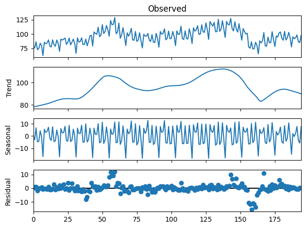
As in FPP2, we are going to build an ARIMA model on the seasonally adjusted data.

ee_stl = STL(ee.elecequip.values, period=12, robust=True).fit()
ee_stl.plot();

../_images/3a84786bcdc1ec170fedb5390010a7f5a5c491fc22abec136d67ee131934b5bc.png

from pmdarima import auto_arima, model_selection


ee_adj = ee_stl.observed - ee_stl.seasonal
ee_train, ee_test = model_selection.train_test_split(ee_adj, train_size=150)
ee_arima = auto_arima(ee_train, error_action='ignore', trace=True,
                      suppress_warnings=True, maxiter=10,
                      seasonal=False)

Performing stepwise search to minimize aic
 ARIMA(2,1,2)(0,0,0)[0] intercept   : AIC=707.575, Time=0.07 sec
 ARIMA(0,1,0)(0,0,0)[0] intercept   : AIC=724.165, Time=0.01 sec
 ARIMA(1,1,0)(0,0,0)[0] intercept   : AIC=715.304, Time=0.02 sec
 ARIMA(0,1,1)(0,0,0)[0] intercept   : AIC=713.256, Time=0.02 sec
 ARIMA(0,1,0)(0,0,0)[0]             : AIC=722.821, Time=0.01 sec
 ARIMA(1,1,2)(0,0,0)[0] intercept   : AIC=712.176, Time=0.05 sec

 ARIMA(2,1,1)(0,0,0)[0] intercept   : AIC=707.187, Time=0.05 sec
 ARIMA(1,1,1)(0,0,0)[0] intercept   : AIC=715.144, Time=0.03 sec
 ARIMA(2,1,0)(0,0,0)[0] intercept   : AIC=710.610, Time=0.03 sec
 ARIMA(3,1,1)(0,0,0)[0] intercept   : AIC=703.640, Time=0.06 sec
 ARIMA(3,1,0)(0,0,0)[0] intercept   : AIC=703.060, Time=0.04 sec

 ARIMA(4,1,0)(0,0,0)[0] intercept   : AIC=704.363, Time=0.06 sec
 ARIMA(4,1,1)(0,0,0)[0] intercept   : AIC=705.507, Time=0.07 sec
 ARIMA(3,1,0)(0,0,0)[0]             : AIC=702.067, Time=0.03 sec
 ARIMA(2,1,0)(0,0,0)[0]             : AIC=710.534, Time=0.02 sec
 ARIMA(4,1,0)(0,0,0)[0]             : AIC=703.193, Time=0.03 sec
 ARIMA(3,1,1)(0,0,0)[0]             : AIC=702.190, Time=0.04 sec

 ARIMA(2,1,1)(0,0,0)[0]             : AIC=706.917, Time=0.03 sec
 ARIMA(4,1,1)(0,0,0)[0]             : AIC=704.063, Time=0.05 sec

Best model:  ARIMA(3,1,0)(0,0,0)[0]          
Total fit time: 0.732 seconds

pmdarima yields a ARIMA(3,1,0) model with an AIC = 702. The example in FPP2 manually selected ARIMA(3,1,1). Let’s look at the predictions.

ee_predict, ee_ci = ee_arima.predict(ee_test.shape[0], return_conf_int=True)

ee_forecast = (
    pd.DataFrame(
        {
            "predicted": ee_predict,
            "actual": ee_test.flatten(),
        }
    )
    .join(pd.DataFrame(ee_ci).rename(columns={0: "lower_ci", 1: "upper_ci"}))
#     .stack()
    .reset_index()
#     .rename(columns={"level_0": "index", "level_1": "label"})
)
line_predicted_elec = (
    alt.Chart(ee_forecast)
    .mark_line()
    .encode(x="index:O", y="predicted:Q")
    .properties(width=800)
)
line_actual_elec = line_predicted_elec.mark_line(color='orange').encode(x="index:O", y="actual")
band_elec = line_predicted_elec.mark_area(opacity=0.5).encode(x="index", y="lower_ci:Q", y2="upper_ci:Q")

#TODO: fix top x-axis
line_predicted_elec + line_actual_elec + band_elec

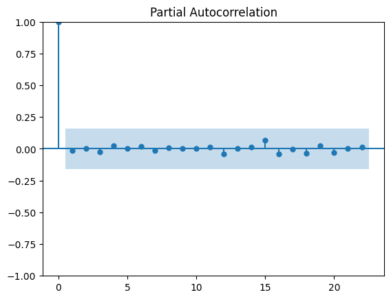
from statsmodels.graphics.tsaplots import plot_acf, plot_pacf
ee_residuals = ee_arima.predict_in_sample() - ee_train
plot_acf(ee_residuals);

../_images/fe5ca9c20d1e2b2f688cc4189a88a3e6a097b4cf47942a752031cab27f7645aa.png

plot_pacf(ee_residuals, method='ywm');

../_images/b6ab70a636d9a48e4b37b1c80dfa1fba7804c9e8514af41cc87848a6e5314d46.png

#TODO: weird outlier at -80?
alt.Chart(pd.DataFrame({"residuals": ee_residuals})).mark_bar().encode(
    alt.X("residuals:Q", bin=alt.Bin(maxbins=30)), y="count():Q"
)