Chapter 15 – Processing Sequences Using RNNs and CNNs#
This notebook contains all the sample code in chapter 15.
Setup#
First, let’s import a few common modules, ensure MatplotLib plots figures inline and prepare a function to save the figures. We also check that Python 3.5 or later is installed (although Python 2.x may work, it is deprecated so we strongly recommend you use Python 3 instead), as well as Scikit-Learn ≥0.20 and TensorFlow ≥2.0.
# Python ≥3.5 is required
import sys
assert sys.version_info >= (3, 5)

# Is this notebook running on Colab or Kaggle?
IS_COLAB = "google.colab" in sys.modules
IS_KAGGLE = "kaggle_secrets" in sys.modules

# Scikit-Learn ≥0.20 is required
import sklearn
assert sklearn.__version__ >= "0.20"

# TensorFlow ≥2.0 is required
import tensorflow as tf
from tensorflow import keras
assert tf.__version__ >= "2.0"

if not tf.config.list_physical_devices('GPU'):
    print("No GPU was detected. LSTMs and CNNs can be very slow without a GPU.")
    if IS_COLAB:
        print("Go to Runtime > Change runtime and select a GPU hardware accelerator.")
    if IS_KAGGLE:
        print("Go to Settings > Accelerator and select GPU.")

# Common imports
import numpy as np
import os
from pathlib import Path

# to make this notebook's output stable across runs
np.random.seed(42)
tf.random.set_seed(42)

# To plot pretty figures
%matplotlib inline
import matplotlib as mpl
import matplotlib.pyplot as plt
mpl.rc('axes', labelsize=14)
mpl.rc('xtick', labelsize=12)
mpl.rc('ytick', labelsize=12)

# Where to save the figures
PROJECT_ROOT_DIR = "."
CHAPTER_ID = "rnn"
IMAGES_PATH = os.path.join(PROJECT_ROOT_DIR, "images", CHAPTER_ID)
os.makedirs(IMAGES_PATH, exist_ok=True)

def save_fig(fig_id, tight_layout=True, fig_extension="png", resolution=300):
    path = os.path.join(IMAGES_PATH, fig_id + "." + fig_extension)
    print("Saving figure", fig_id)
    if tight_layout:
        plt.tight_layout()
    plt.savefig(path, format=fig_extension, dpi=resolution)
No GPU was detected. LSTMs and CNNs can be very slow without a GPU.
Basic RNNs#
Generate the Dataset#
def generate_time_series(batch_size, n_steps):
    freq1, freq2, offsets1, offsets2 = np.random.rand(4, batch_size, 1)
    time = np.linspace(0, 1, n_steps)
    series = 0.5 * np.sin((time - offsets1) * (freq1 * 10 + 10))  #   wave 1
    series += 0.2 * np.sin((time - offsets2) * (freq2 * 20 + 20)) # + wave 2
    series += 0.1 * (np.random.rand(batch_size, n_steps) - 0.5)   # + noise
    return series[..., np.newaxis].astype(np.float32)
np.random.seed(42)

n_steps = 50
series = generate_time_series(10000, n_steps + 1)
X_train, y_train = series[:7000, :n_steps], series[:7000, -1]
X_valid, y_valid = series[7000:9000, :n_steps], series[7000:9000, -1]
X_test, y_test = series[9000:, :n_steps], series[9000:, -1]
X_train.shape, y_train.shape
((7000, 50, 1), (7000, 1))
def plot_series(series, y=None, y_pred=None, x_label="$t$", y_label="$x(t)$", legend=True):
    plt.plot(series, ".-")
    if y is not None:
        plt.plot(n_steps, y, "bo", label="Target")
    if y_pred is not None:
        plt.plot(n_steps, y_pred, "rx", markersize=10, label="Prediction")
    plt.grid(True)
    if x_label:
        plt.xlabel(x_label, fontsize=16)
    if y_label:
        plt.ylabel(y_label, fontsize=16, rotation=0)
    plt.hlines(0, 0, 100, linewidth=1)
    plt.axis([0, n_steps + 1, -1, 1])
    if legend and (y or y_pred):
        plt.legend(fontsize=14, loc="upper left")

fig, axes = plt.subplots(nrows=1, ncols=3, sharey=True, figsize=(12, 4))
for col in range(3):
    plt.sca(axes[col])
    plot_series(X_valid[col, :, 0], y_valid[col, 0],
                y_label=("$x(t)$" if col==0 else None),
                legend=(col == 0))
save_fig("time_series_plot")
plt.show()
Saving figure time_series_plot
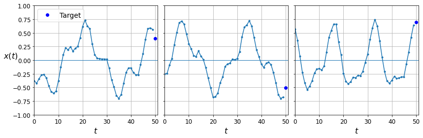
Note: in this notebook, the blue dots represent targets, and red crosses represent predictions. In the book, I first used blue crosses for targets and red dots for predictions, then I reversed this later in the chapter. Sorry if this caused some confusion.
Computing Some Baselines#
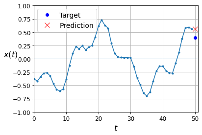
Naive predictions (just predict the last observed value):
y_pred = X_valid[:, -1]
np.mean(keras.losses.mean_squared_error(y_valid, y_pred))
0.020211367
plot_series(X_valid[0, :, 0], y_valid[0, 0], y_pred[0, 0])
plt.show()
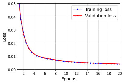
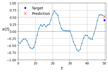
Linear predictions:
np.random.seed(42)
tf.random.set_seed(42)

model = keras.models.Sequential([
    keras.layers.Flatten(input_shape=[50, 1]),
    keras.layers.Dense(1)
])

model.compile(loss="mse", optimizer="adam")
history = model.fit(X_train, y_train, epochs=20,
                    validation_data=(X_valid, y_valid))
Epoch 1/20
219/219 [==============================] - 1s 3ms/step - loss: 0.1398 - val_loss: 0.0545
Epoch 2/20
219/219 [==============================] - 0s 690us/step - loss: 0.0443 - val_loss: 0.0266
Epoch 3/20
219/219 [==============================] - 0s 631us/step - loss: 0.0237 - val_loss: 0.0157
Epoch 4/20
219/219 [==============================] - 0s 738us/step - loss: 0.0142 - val_loss: 0.0116
Epoch 5/20
219/219 [==============================] - 0s 740us/step - loss: 0.0110 - val_loss: 0.0098
Epoch 6/20
219/219 [==============================] - 0s 615us/step - loss: 0.0093 - val_loss: 0.0087
Epoch 7/20
219/219 [==============================] - 0s 590us/step - loss: 0.0083 - val_loss: 0.0079
Epoch 8/20
219/219 [==============================] - 0s 581us/step - loss: 0.0074 - val_loss: 0.0071
Epoch 9/20
219/219 [==============================] - 0s 562us/step - loss: 0.0064 - val_loss: 0.0066
Epoch 10/20
219/219 [==============================] - 0s 570us/step - loss: 0.0063 - val_loss: 0.0062
Epoch 11/20
219/219 [==============================] - 0s 576us/step - loss: 0.0059 - val_loss: 0.0057
Epoch 12/20
219/219 [==============================] - 0s 645us/step - loss: 0.0054 - val_loss: 0.0055
Epoch 13/20
219/219 [==============================] - 0s 578us/step - loss: 0.0052 - val_loss: 0.0052
Epoch 14/20
219/219 [==============================] - 0s 596us/step - loss: 0.0050 - val_loss: 0.0049
Epoch 15/20
219/219 [==============================] - 0s 707us/step - loss: 0.0048 - val_loss: 0.0048
Epoch 16/20
219/219 [==============================] - 0s 635us/step - loss: 0.0046 - val_loss: 0.0048
Epoch 17/20
219/219 [==============================] - 0s 604us/step - loss: 0.0046 - val_loss: 0.0045
Epoch 18/20
219/219 [==============================] - 0s 647us/step - loss: 0.0043 - val_loss: 0.0044
Epoch 19/20
219/219 [==============================] - 0s 659us/step - loss: 0.0042 - val_loss: 0.0043
Epoch 20/20
219/219 [==============================] - 0s 769us/step - loss: 0.0043 - val_loss: 0.0042
model.evaluate(X_valid, y_valid)
63/63 [==============================] - 0s 414us/step - loss: 0.0042
0.004168087150901556
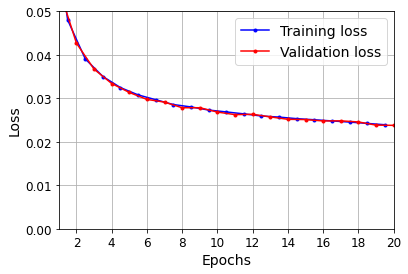
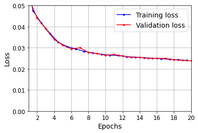
def plot_learning_curves(loss, val_loss):
    plt.plot(np.arange(len(loss)) + 0.5, loss, "b.-", label="Training loss")
    plt.plot(np.arange(len(val_loss)) + 1, val_loss, "r.-", label="Validation loss")
    plt.gca().xaxis.set_major_locator(mpl.ticker.MaxNLocator(integer=True))
    plt.axis([1, 20, 0, 0.05])
    plt.legend(fontsize=14)
    plt.xlabel("Epochs")
    plt.ylabel("Loss")
    plt.grid(True)

plot_learning_curves(history.history["loss"], history.history["val_loss"])
plt.show()
y_pred = model.predict(X_valid)
plot_series(X_valid[0, :, 0], y_valid[0, 0], y_pred[0, 0])
plt.show()
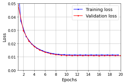
Using a Simple RNN#
np.random.seed(42)
tf.random.set_seed(42)

model = keras.models.Sequential([
    keras.layers.SimpleRNN(1, input_shape=[None, 1])
])

optimizer = keras.optimizers.Adam(learning_rate=0.005)
model.compile(loss="mse", optimizer=optimizer)
history = model.fit(X_train, y_train, epochs=20,
                    validation_data=(X_valid, y_valid))
Epoch 1/20
219/219 [==============================] - 2s 5ms/step - loss: 0.1554 - val_loss: 0.0489
Epoch 2/20
219/219 [==============================] - 1s 4ms/step - loss: 0.0409 - val_loss: 0.0296
Epoch 3/20
219/219 [==============================] - 1s 4ms/step - loss: 0.0277 - val_loss: 0.0218
Epoch 4/20
219/219 [==============================] - 1s 4ms/step - loss: 0.0208 - val_loss: 0.0177
Epoch 5/20
219/219 [==============================] - 1s 4ms/step - loss: 0.0174 - val_loss: 0.0151
Epoch 6/20
219/219 [==============================] - 1s 4ms/step - loss: 0.0146 - val_loss: 0.0134
Epoch 7/20
219/219 [==============================] - 1s 4ms/step - loss: 0.0138 - val_loss: 0.0123
Epoch 8/20
219/219 [==============================] - 1s 4ms/step - loss: 0.0128 - val_loss: 0.0116
Epoch 9/20
219/219 [==============================] - 1s 4ms/step - loss: 0.0118 - val_loss: 0.0112
Epoch 10/20
219/219 [==============================] - 1s 4ms/step - loss: 0.0117 - val_loss: 0.0110
Epoch 11/20
219/219 [==============================] - 1s 4ms/step - loss: 0.0112 - val_loss: 0.0109
Epoch 12/20
219/219 [==============================] - 1s 4ms/step - loss: 0.0115 - val_loss: 0.0109
Epoch 13/20
219/219 [==============================] - 1s 4ms/step - loss: 0.0114 - val_loss: 0.0109
Epoch 14/20
219/219 [==============================] - 1s 4ms/step - loss: 0.0114 - val_loss: 0.0109
Epoch 15/20
219/219 [==============================] - 1s 4ms/step - loss: 0.0113 - val_loss: 0.0109
Epoch 16/20
219/219 [==============================] - 1s 4ms/step - loss: 0.0114 - val_loss: 0.0109
Epoch 17/20
219/219 [==============================] - 1s 4ms/step - loss: 0.0114 - val_loss: 0.0109
Epoch 18/20
219/219 [==============================] - 1s 4ms/step - loss: 0.0115 - val_loss: 0.0109
Epoch 19/20
219/219 [==============================] - 1s 5ms/step - loss: 0.0115 - val_loss: 0.0109
Epoch 20/20
219/219 [==============================] - 1s 4ms/step - loss: 0.0116 - val_loss: 0.0109
model.evaluate(X_valid, y_valid)
63/63 [==============================] - 0s 2ms/step - loss: 0.0109
0.010881561785936356
plot_learning_curves(history.history["loss"], history.history["val_loss"])
plt.show()
y_pred = model.predict(X_valid)
plot_series(X_valid[0, :, 0], y_valid[0, 0], y_pred[0, 0])
plt.show()

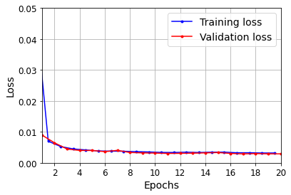
Deep RNNs#
np.random.seed(42)
tf.random.set_seed(42)

model = keras.models.Sequential([
    keras.layers.SimpleRNN(20, return_sequences=True, input_shape=[None, 1]),
    keras.layers.SimpleRNN(20, return_sequences=True),
    keras.layers.SimpleRNN(1)
])

model.compile(loss="mse", optimizer="adam")
history = model.fit(X_train, y_train, epochs=20,
                    validation_data=(X_valid, y_valid))
Epoch 1/20
219/219 [==============================] - 5s 17ms/step - loss: 0.1324 - val_loss: 0.0090
Epoch 2/20
219/219 [==============================] - 3s 15ms/step - loss: 0.0078 - val_loss: 0.0065
Epoch 3/20
219/219 [==============================] - 3s 15ms/step - loss: 0.0057 - val_loss: 0.0045
Epoch 4/20
219/219 [==============================] - 3s 15ms/step - loss: 0.0045 - val_loss: 0.0040
Epoch 5/20
219/219 [==============================] - 3s 15ms/step - loss: 0.0044 - val_loss: 0.0040
Epoch 6/20
219/219 [==============================] - 3s 15ms/step - loss: 0.0038 - val_loss: 0.0036
Epoch 7/20
219/219 [==============================] - 3s 15ms/step - loss: 0.0036 - val_loss: 0.0040
Epoch 8/20
219/219 [==============================] - 3s 15ms/step - loss: 0.0038 - val_loss: 0.0033
Epoch 9/20
219/219 [==============================] - 3s 15ms/step - loss: 0.0037 - val_loss: 0.0032
Epoch 10/20
219/219 [==============================] - 3s 15ms/step - loss: 0.0035 - val_loss: 0.0031
Epoch 11/20
219/219 [==============================] - 3s 15ms/step - loss: 0.0034 - val_loss: 0.0030
Epoch 12/20
219/219 [==============================] - 3s 15ms/step - loss: 0.0033 - val_loss: 0.0031
Epoch 13/20
219/219 [==============================] - 3s 15ms/step - loss: 0.0034 - val_loss: 0.0031
Epoch 14/20
219/219 [==============================] - 3s 15ms/step - loss: 0.0034 - val_loss: 0.0032
Epoch 15/20
219/219 [==============================] - 3s 15ms/step - loss: 0.0034 - val_loss: 0.0033
Epoch 16/20
219/219 [==============================] - 3s 15ms/step - loss: 0.0037 - val_loss: 0.0030
Epoch 17/20
219/219 [==============================] - 3s 14ms/step - loss: 0.0034 - val_loss: 0.0029
Epoch 18/20
219/219 [==============================] - 3s 14ms/step - loss: 0.0031 - val_loss: 0.0030
Epoch 19/20
219/219 [==============================] - 3s 14ms/step - loss: 0.0032 - val_loss: 0.0029
Epoch 20/20
219/219 [==============================] - 3s 14ms/step - loss: 0.0033 - val_loss: 0.0029
model.evaluate(X_valid, y_valid)
63/63 [==============================] - 0s 3ms/step - loss: 0.0029
0.002910564187914133
plot_learning_curves(history.history["loss"], history.history["val_loss"])
plt.show()
y_pred = model.predict(X_valid)
plot_series(X_valid[0, :, 0], y_valid[0, 0], y_pred[0, 0])
plt.show()

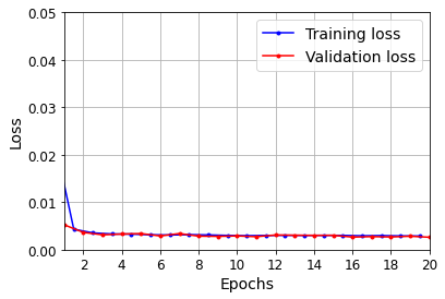
Make the second SimpleRNN layer return only the last output:
np.random.seed(42)
tf.random.set_seed(42)

model = keras.models.Sequential([
    keras.layers.SimpleRNN(20, return_sequences=True, input_shape=[None, 1]),
    keras.layers.SimpleRNN(20),
    keras.layers.Dense(1)
])

model.compile(loss="mse", optimizer="adam")
history = model.fit(X_train, y_train, epochs=20,
                    validation_data=(X_valid, y_valid))
Epoch 1/20
219/219 [==============================] - 3s 12ms/step - loss: 0.0566 - val_loss: 0.0052
Epoch 2/20
219/219 [==============================] - 2s 11ms/step - loss: 0.0048 - val_loss: 0.0036
Epoch 3/20
219/219 [==============================] - 2s 11ms/step - loss: 0.0036 - val_loss: 0.0031
Epoch 4/20
219/219 [==============================] - 2s 11ms/step - loss: 0.0033 - val_loss: 0.0033
Epoch 5/20
219/219 [==============================] - 2s 11ms/step - loss: 0.0033 - val_loss: 0.0034
Epoch 6/20
219/219 [==============================] - 3s 11ms/step - loss: 0.0031 - val_loss: 0.0029
Epoch 7/20
219/219 [==============================] - 2s 11ms/step - loss: 0.0030 - val_loss: 0.0034
Epoch 8/20
219/219 [==============================] - 3s 12ms/step - loss: 0.0033 - val_loss: 0.0028
Epoch 9/20
219/219 [==============================] - 3s 12ms/step - loss: 0.0031 - val_loss: 0.0028
Epoch 10/20
219/219 [==============================] - 3s 12ms/step - loss: 0.0029 - val_loss: 0.0029
Epoch 11/20
219/219 [==============================] - 3s 12ms/step - loss: 0.0029 - val_loss: 0.0027
Epoch 12/20
219/219 [==============================] - 3s 12ms/step - loss: 0.0029 - val_loss: 0.0031
Epoch 13/20
219/219 [==============================] - 3s 12ms/step - loss: 0.0029 - val_loss: 0.0031
Epoch 14/20
219/219 [==============================] - 2s 11ms/step - loss: 0.0031 - val_loss: 0.0030
Epoch 15/20
219/219 [==============================] - 2s 11ms/step - loss: 0.0030 - val_loss: 0.0030
Epoch 16/20
219/219 [==============================] - 2s 11ms/step - loss: 0.0030 - val_loss: 0.0027
Epoch 17/20
219/219 [==============================] - 2s 11ms/step - loss: 0.0030 - val_loss: 0.0028
Epoch 18/20
219/219 [==============================] - 2s 11ms/step - loss: 0.0029 - val_loss: 0.0027
Epoch 19/20
219/219 [==============================] - 2s 11ms/step - loss: 0.0029 - val_loss: 0.0028
Epoch 20/20
219/219 [==============================] - 2s 11ms/step - loss: 0.0030 - val_loss: 0.0026
model.evaluate(X_valid, y_valid)
63/63 [==============================] - 0s 3ms/step - loss: 0.0026
0.002623623702675104
plot_learning_curves(history.history["loss"], history.history["val_loss"])
plt.show()
y_pred = model.predict(X_valid)
plot_series(X_valid[0, :, 0], y_valid[0, 0], y_pred[0, 0])
plt.show()
Forecasting Several Steps Ahead#
np.random.seed(43) # not 42, as it would give the first series in the train set

series = generate_time_series(1, n_steps + 10)
X_new, Y_new = series[:, :n_steps], series[:, n_steps:]
X = X_new
for step_ahead in range(10):
    y_pred_one = model.predict(X[:, step_ahead:])[:, np.newaxis, :]
    X = np.concatenate([X, y_pred_one], axis=1)

Y_pred = X[:, n_steps:]
Y_pred.shape
(1, 10, 1)
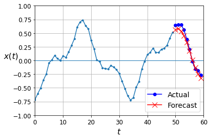
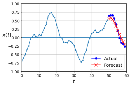
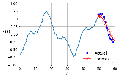
def plot_multiple_forecasts(X, Y, Y_pred):
    n_steps = X.shape[1]
    ahead = Y.shape[1]
    plot_series(X[0, :, 0])
    plt.plot(np.arange(n_steps, n_steps + ahead), Y[0, :, 0], "bo-", label="Actual")
    plt.plot(np.arange(n_steps, n_steps + ahead), Y_pred[0, :, 0], "rx-", label="Forecast", markersize=10)
    plt.axis([0, n_steps + ahead, -1, 1])
    plt.legend(fontsize=14)

plot_multiple_forecasts(X_new, Y_new, Y_pred)
save_fig("forecast_ahead_plot")
plt.show()
Saving figure forecast_ahead_plot
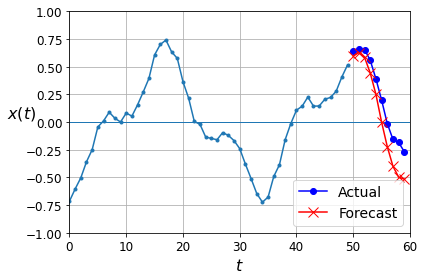
Now let’s use this model to predict the next 10 values. We first need to regenerate the sequences with 9 more time steps.
np.random.seed(42)

n_steps = 50
series = generate_time_series(10000, n_steps + 10)
X_train, Y_train = series[:7000, :n_steps], series[:7000, -10:, 0]
X_valid, Y_valid = series[7000:9000, :n_steps], series[7000:9000, -10:, 0]
X_test, Y_test = series[9000:, :n_steps], series[9000:, -10:, 0]
Now let’s predict the next 10 values one by one:
X = X_valid
for step_ahead in range(10):
    y_pred_one = model.predict(X)[:, np.newaxis, :]
    X = np.concatenate([X, y_pred_one], axis=1)

Y_pred = X[:, n_steps:, 0]
Y_pred.shape
(2000, 10)
np.mean(keras.metrics.mean_squared_error(Y_valid, Y_pred))
0.027510857
Let’s compare this performance with some baselines: naive predictions and a simple linear model:
Y_naive_pred = np.tile(X_valid[:, -1], 10) # take the last time step value, and repeat it 10 times
np.mean(keras.metrics.mean_squared_error(Y_valid, Y_naive_pred))
0.25697407
np.random.seed(42)
tf.random.set_seed(42)

model = keras.models.Sequential([
    keras.layers.Flatten(input_shape=[50, 1]),
    keras.layers.Dense(10)
])

model.compile(loss="mse", optimizer="adam")
history = model.fit(X_train, Y_train, epochs=20,
                    validation_data=(X_valid, Y_valid))
Epoch 1/20
219/219 [==============================] - 0s 1ms/step - loss: 0.2186 - val_loss: 0.0606
Epoch 2/20
219/219 [==============================] - 0s 743us/step - loss: 0.0535 - val_loss: 0.0425
Epoch 3/20
219/219 [==============================] - 0s 727us/step - loss: 0.0406 - val_loss: 0.0353
Epoch 4/20
219/219 [==============================] - 0s 731us/step - loss: 0.0343 - val_loss: 0.0311
Epoch 5/20
219/219 [==============================] - 0s 743us/step - loss: 0.0300 - val_loss: 0.0283
Epoch 6/20
219/219 [==============================] - 0s 721us/step - loss: 0.0278 - val_loss: 0.0264
Epoch 7/20
219/219 [==============================] - 0s 722us/step - loss: 0.0262 - val_loss: 0.0249
Epoch 8/20
219/219 [==============================] - 0s 731us/step - loss: 0.0246 - val_loss: 0.0237
Epoch 9/20
219/219 [==============================] - 0s 725us/step - loss: 0.0236 - val_loss: 0.0229
Epoch 10/20
219/219 [==============================] - 0s 735us/step - loss: 0.0228 - val_loss: 0.0222
Epoch 11/20
219/219 [==============================] - 0s 743us/step - loss: 0.0220 - val_loss: 0.0216
Epoch 12/20
219/219 [==============================] - 0s 733us/step - loss: 0.0214 - val_loss: 0.0212
Epoch 13/20
219/219 [==============================] - 0s 714us/step - loss: 0.0212 - val_loss: 0.0208
Epoch 14/20
219/219 [==============================] - 0s 739us/step - loss: 0.0207 - val_loss: 0.0207
Epoch 15/20
219/219 [==============================] - 0s 712us/step - loss: 0.0207 - val_loss: 0.0202
Epoch 16/20
219/219 [==============================] - 0s 723us/step - loss: 0.0199 - val_loss: 0.0199
Epoch 17/20
219/219 [==============================] - 0s 738us/step - loss: 0.0197 - val_loss: 0.0195
Epoch 18/20
219/219 [==============================] - 0s 715us/step - loss: 0.0190 - val_loss: 0.0192
Epoch 19/20
219/219 [==============================] - 0s 719us/step - loss: 0.0189 - val_loss: 0.0189
Epoch 20/20
219/219 [==============================] - 0s 726us/step - loss: 0.0188 - val_loss: 0.0187
Now let’s create an RNN that predicts all 10 next values at once:
np.random.seed(42)
tf.random.set_seed(42)

model = keras.models.Sequential([
    keras.layers.SimpleRNN(20, return_sequences=True, input_shape=[None, 1]),
    keras.layers.SimpleRNN(20),
    keras.layers.Dense(10)
])

model.compile(loss="mse", optimizer="adam")
history = model.fit(X_train, Y_train, epochs=20,
                    validation_data=(X_valid, Y_valid))
Epoch 1/20
219/219 [==============================] - 3s 12ms/step - loss: 0.1216 - val_loss: 0.0317
Epoch 2/20
219/219 [==============================] - 2s 11ms/step - loss: 0.0294 - val_loss: 0.0200
Epoch 3/20
219/219 [==============================] - 3s 11ms/step - loss: 0.0198 - val_loss: 0.0160
Epoch 4/20
219/219 [==============================] - 2s 11ms/step - loss: 0.0162 - val_loss: 0.0144
Epoch 5/20
219/219 [==============================] - 2s 11ms/step - loss: 0.0144 - val_loss: 0.0118
Epoch 6/20
219/219 [==============================] - 2s 11ms/step - loss: 0.0127 - val_loss: 0.0112
Epoch 7/20
219/219 [==============================] - 2s 11ms/step - loss: 0.0119 - val_loss: 0.0110
Epoch 8/20
219/219 [==============================] - 2s 11ms/step - loss: 0.0114 - val_loss: 0.0103
Epoch 9/20
219/219 [==============================] - 3s 12ms/step - loss: 0.0110 - val_loss: 0.0112
Epoch 10/20
219/219 [==============================] - 2s 11ms/step - loss: 0.0118 - val_loss: 0.0100
Epoch 11/20
219/219 [==============================] - 2s 11ms/step - loss: 0.0109 - val_loss: 0.0103
Epoch 12/20
219/219 [==============================] - 2s 11ms/step - loss: 0.0104 - val_loss: 0.0096
Epoch 13/20
219/219 [==============================] - 2s 11ms/step - loss: 0.0103 - val_loss: 0.0100
Epoch 14/20
219/219 [==============================] - 2s 11ms/step - loss: 0.0101 - val_loss: 0.0103
Epoch 15/20
219/219 [==============================] - 2s 11ms/step - loss: 0.0095 - val_loss: 0.0107
Epoch 16/20
219/219 [==============================] - 2s 11ms/step - loss: 0.0095 - val_loss: 0.0089
Epoch 17/20
219/219 [==============================] - 2s 11ms/step - loss: 0.0092 - val_loss: 0.0111
Epoch 18/20
219/219 [==============================] - 2s 11ms/step - loss: 0.0098 - val_loss: 0.0094
Epoch 19/20
219/219 [==============================] - 2s 11ms/step - loss: 0.0090 - val_loss: 0.0083
Epoch 20/20
219/219 [==============================] - 2s 11ms/step - loss: 0.0092 - val_loss: 0.0085
np.random.seed(43)

series = generate_time_series(1, 50 + 10)
X_new, Y_new = series[:, :50, :], series[:, -10:, :]
Y_pred = model.predict(X_new)[..., np.newaxis]
plot_multiple_forecasts(X_new, Y_new, Y_pred)
plt.show()

Now let’s create an RNN that predicts the next 10 steps at each time step. That is, instead of just forecasting time steps 50 to 59 based on time steps 0 to 49, it will forecast time steps 1 to 10 at time step 0, then time steps 2 to 11 at time step 1, and so on, and finally it will forecast time steps 50 to 59 at the last time step. Notice that the model is causal: when it makes predictions at any time step, it can only see past time steps.
np.random.seed(42)

n_steps = 50
series = generate_time_series(10000, n_steps + 10)
X_train = series[:7000, :n_steps]
X_valid = series[7000:9000, :n_steps]
X_test = series[9000:, :n_steps]
Y = np.empty((10000, n_steps, 10))
for step_ahead in range(1, 10 + 1):
    Y[..., step_ahead - 1] = series[..., step_ahead:step_ahead + n_steps, 0]
Y_train = Y[:7000]
Y_valid = Y[7000:9000]
Y_test = Y[9000:]
X_train.shape, Y_train.shape
((7000, 50, 1), (7000, 50, 10))
np.random.seed(42)
tf.random.set_seed(42)

model = keras.models.Sequential([
    keras.layers.SimpleRNN(20, return_sequences=True, input_shape=[None, 1]),
    keras.layers.SimpleRNN(20, return_sequences=True),
    keras.layers.TimeDistributed(keras.layers.Dense(10))
])

def last_time_step_mse(Y_true, Y_pred):
    return keras.metrics.mean_squared_error(Y_true[:, -1], Y_pred[:, -1])

model.compile(loss="mse", optimizer=keras.optimizers.Adam(learning_rate=0.01), metrics=[last_time_step_mse])
history = model.fit(X_train, Y_train, epochs=20,
                    validation_data=(X_valid, Y_valid))
Epoch 1/20
219/219 [==============================] - 4s 12ms/step - loss: 0.0705 - last_time_step_mse: 0.0621 - val_loss: 0.0429 - val_last_time_step_mse: 0.0324
Epoch 2/20
219/219 [==============================] - 3s 12ms/step - loss: 0.0413 - last_time_step_mse: 0.0301 - val_loss: 0.0366 - val_last_time_step_mse: 0.0264
Epoch 3/20
219/219 [==============================] - 3s 11ms/step - loss: 0.0333 - last_time_step_mse: 0.0223 - val_loss: 0.0343 - val_last_time_step_mse: 0.0244
Epoch 4/20
219/219 [==============================] - 2s 11ms/step - loss: 0.0306 - last_time_step_mse: 0.0200 - val_loss: 0.0284 - val_last_time_step_mse: 0.0164
Epoch 5/20
219/219 [==============================] - 2s 11ms/step - loss: 0.0281 - last_time_step_mse: 0.0167 - val_loss: 0.0282 - val_last_time_step_mse: 0.0196
Epoch 6/20
219/219 [==============================] - 3s 11ms/step - loss: 0.0259 - last_time_step_mse: 0.0137 - val_loss: 0.0215 - val_last_time_step_mse: 0.0081
Epoch 7/20
219/219 [==============================] - 2s 11ms/step - loss: 0.0234 - last_time_step_mse: 0.0105 - val_loss: 0.0220 - val_last_time_step_mse: 0.0089
Epoch 8/20
219/219 [==============================] - 2s 11ms/step - loss: 0.0216 - last_time_step_mse: 0.0085 - val_loss: 0.0217 - val_last_time_step_mse: 0.0091
Epoch 9/20
219/219 [==============================] - 3s 12ms/step - loss: 0.0214 - last_time_step_mse: 0.0089 - val_loss: 0.0202 - val_last_time_step_mse: 0.0074
Epoch 10/20
219/219 [==============================] - 3s 12ms/step - loss: 0.0210 - last_time_step_mse: 0.0085 - val_loss: 0.0211 - val_last_time_step_mse: 0.0086
Epoch 11/20
219/219 [==============================] - 3s 11ms/step - loss: 0.0203 - last_time_step_mse: 0.0078 - val_loss: 0.0201 - val_last_time_step_mse: 0.0078
Epoch 12/20
219/219 [==============================] - 2s 11ms/step - loss: 0.0203 - last_time_step_mse: 0.0079 - val_loss: 0.0194 - val_last_time_step_mse: 0.0073
Epoch 13/20
219/219 [==============================] - 2s 11ms/step - loss: 0.0198 - last_time_step_mse: 0.0074 - val_loss: 0.0209 - val_last_time_step_mse: 0.0085
Epoch 14/20
219/219 [==============================] - 3s 12ms/step - loss: 0.0197 - last_time_step_mse: 0.0073 - val_loss: 0.0189 - val_last_time_step_mse: 0.0067
Epoch 15/20
219/219 [==============================] - 3s 12ms/step - loss: 0.0192 - last_time_step_mse: 0.0072 - val_loss: 0.0182 - val_last_time_step_mse: 0.0066
Epoch 16/20
219/219 [==============================] - 2s 11ms/step - loss: 0.0187 - last_time_step_mse: 0.0066 - val_loss: 0.0196 - val_last_time_step_mse: 0.0095
Epoch 17/20
219/219 [==============================] - 2s 11ms/step - loss: 0.0187 - last_time_step_mse: 0.0067 - val_loss: 0.0185 - val_last_time_step_mse: 0.0072
Epoch 18/20
219/219 [==============================] - 2s 11ms/step - loss: 0.0186 - last_time_step_mse: 0.0067 - val_loss: 0.0179 - val_last_time_step_mse: 0.0064
Epoch 19/20
219/219 [==============================] - 3s 11ms/step - loss: 0.0185 - last_time_step_mse: 0.0068 - val_loss: 0.0172 - val_last_time_step_mse: 0.0058
Epoch 20/20
219/219 [==============================] - 2s 11ms/step - loss: 0.0181 - last_time_step_mse: 0.0066 - val_loss: 0.0205 - val_last_time_step_mse: 0.0096
np.random.seed(43)

series = generate_time_series(1, 50 + 10)
X_new, Y_new = series[:, :50, :], series[:, 50:, :]
Y_pred = model.predict(X_new)[:, -1][..., np.newaxis]
plot_multiple_forecasts(X_new, Y_new, Y_pred)
plt.show()
Deep RNN with Batch Norm#
np.random.seed(42)
tf.random.set_seed(42)

model = keras.models.Sequential([
    keras.layers.SimpleRNN(20, return_sequences=True, input_shape=[None, 1]),
    keras.layers.BatchNormalization(),
    keras.layers.SimpleRNN(20, return_sequences=True),
    keras.layers.BatchNormalization(),
    keras.layers.TimeDistributed(keras.layers.Dense(10))
])

model.compile(loss="mse", optimizer="adam", metrics=[last_time_step_mse])
history = model.fit(X_train, Y_train, epochs=20,
                    validation_data=(X_valid, Y_valid))
Epoch 1/20
219/219 [==============================] - 4s 13ms/step - loss: 0.4750 - last_time_step_mse: 0.5027 - val_loss: 0.0877 - val_last_time_step_mse: 0.0832
Epoch 2/20
219/219 [==============================] - 3s 12ms/step - loss: 0.0561 - last_time_step_mse: 0.0468 - val_loss: 0.0549 - val_last_time_step_mse: 0.0462
Epoch 3/20
219/219 [==============================] - 3s 12ms/step - loss: 0.0486 - last_time_step_mse: 0.0394 - val_loss: 0.0451 - val_last_time_step_mse: 0.0358
Epoch 4/20
219/219 [==============================] - 3s 12ms/step - loss: 0.0443 - last_time_step_mse: 0.0344 - val_loss: 0.0418 - val_last_time_step_mse: 0.0314
Epoch 5/20
219/219 [==============================] - 3s 12ms/step - loss: 0.0414 - last_time_step_mse: 0.0315 - val_loss: 0.0391 - val_last_time_step_mse: 0.0287
Epoch 6/20
219/219 [==============================] - 3s 12ms/step - loss: 0.0391 - last_time_step_mse: 0.0281 - val_loss: 0.0379 - val_last_time_step_mse: 0.0273
Epoch 7/20
219/219 [==============================] - 3s 12ms/step - loss: 0.0370 - last_time_step_mse: 0.0257 - val_loss: 0.0367 - val_last_time_step_mse: 0.0248
Epoch 8/20
219/219 [==============================] - 3s 12ms/step - loss: 0.0352 - last_time_step_mse: 0.0236 - val_loss: 0.0363 - val_last_time_step_mse: 0.0249
Epoch 9/20
219/219 [==============================] - 3s 12ms/step - loss: 0.0340 - last_time_step_mse: 0.0224 - val_loss: 0.0332 - val_last_time_step_mse: 0.0208
Epoch 10/20
219/219 [==============================] - 3s 12ms/step - loss: 0.0332 - last_time_step_mse: 0.0213 - val_loss: 0.0335 - val_last_time_step_mse: 0.0214
Epoch 11/20
219/219 [==============================] - 3s 12ms/step - loss: 0.0325 - last_time_step_mse: 0.0214 - val_loss: 0.0323 - val_last_time_step_mse: 0.0203
Epoch 12/20
219/219 [==============================] - 3s 12ms/step - loss: 0.0316 - last_time_step_mse: 0.0196 - val_loss: 0.0333 - val_last_time_step_mse: 0.0210
Epoch 13/20
219/219 [==============================] - 3s 12ms/step - loss: 0.0312 - last_time_step_mse: 0.0192 - val_loss: 0.0310 - val_last_time_step_mse: 0.0187
Epoch 14/20
219/219 [==============================] - 3s 12ms/step - loss: 0.0308 - last_time_step_mse: 0.0187 - val_loss: 0.0310 - val_last_time_step_mse: 0.0189
Epoch 15/20
219/219 [==============================] - 3s 12ms/step - loss: 0.0302 - last_time_step_mse: 0.0183 - val_loss: 0.0298 - val_last_time_step_mse: 0.0178
Epoch 16/20
219/219 [==============================] - 3s 12ms/step - loss: 0.0298 - last_time_step_mse: 0.0177 - val_loss: 0.0293 - val_last_time_step_mse: 0.0174
Epoch 17/20
219/219 [==============================] - 3s 12ms/step - loss: 0.0294 - last_time_step_mse: 0.0173 - val_loss: 0.0315 - val_last_time_step_mse: 0.0200
Epoch 18/20
219/219 [==============================] - 3s 12ms/step - loss: 0.0289 - last_time_step_mse: 0.0167 - val_loss: 0.0295 - val_last_time_step_mse: 0.0174
Epoch 19/20
219/219 [==============================] - 3s 12ms/step - loss: 0.0287 - last_time_step_mse: 0.0168 - val_loss: 0.0290 - val_last_time_step_mse: 0.0163
Epoch 20/20
219/219 [==============================] - 3s 12ms/step - loss: 0.0281 - last_time_step_mse: 0.0161 - val_loss: 0.0288 - val_last_time_step_mse: 0.0164
Deep RNNs with Layer Norm#
from tensorflow.keras.layers import LayerNormalization
class LNSimpleRNNCell(keras.layers.Layer):
    def __init__(self, units, activation="tanh", **kwargs):
        super().__init__(**kwargs)
        self.state_size = units
        self.output_size = units
        self.simple_rnn_cell = keras.layers.SimpleRNNCell(units,
                                                          activation=None)
        self.layer_norm = LayerNormalization()
        self.activation = keras.activations.get(activation)
    def get_initial_state(self, inputs=None, batch_size=None, dtype=None):
        if inputs is not None:
            batch_size = tf.shape(inputs)[0]
            dtype = inputs.dtype
        return [tf.zeros([batch_size, self.state_size], dtype=dtype)]
    def call(self, inputs, states):
        outputs, new_states = self.simple_rnn_cell(inputs, states)
        norm_outputs = self.activation(self.layer_norm(outputs))
        return norm_outputs, [norm_outputs]
np.random.seed(42)
tf.random.set_seed(42)

model = keras.models.Sequential([
    keras.layers.RNN(LNSimpleRNNCell(20), return_sequences=True,
                     input_shape=[None, 1]),
    keras.layers.RNN(LNSimpleRNNCell(20), return_sequences=True),
    keras.layers.TimeDistributed(keras.layers.Dense(10))
])

model.compile(loss="mse", optimizer="adam", metrics=[last_time_step_mse])
history = model.fit(X_train, Y_train, epochs=20,
                    validation_data=(X_valid, Y_valid))
Epoch 1/20
219/219 [==============================] - 7s 26ms/step - loss: 0.2860 - last_time_step_mse: 0.2822 - val_loss: 0.0734 - val_last_time_step_mse: 0.0624
Epoch 2/20
219/219 [==============================] - 5s 25ms/step - loss: 0.0679 - last_time_step_mse: 0.0546 - val_loss: 0.0566 - val_last_time_step_mse: 0.0423
Epoch 3/20
219/219 [==============================] - 5s 25ms/step - loss: 0.0553 - last_time_step_mse: 0.0406 - val_loss: 0.0509 - val_last_time_step_mse: 0.0342
Epoch 4/20
219/219 [==============================] - 5s 25ms/step - loss: 0.0485 - last_time_step_mse: 0.0328 - val_loss: 0.0442 - val_last_time_step_mse: 0.0286
Epoch 5/20
219/219 [==============================] - 5s 24ms/step - loss: 0.0435 - last_time_step_mse: 0.0281 - val_loss: 0.0418 - val_last_time_step_mse: 0.0258
Epoch 6/20
219/219 [==============================] - 5s 24ms/step - loss: 0.0404 - last_time_step_mse: 0.0249 - val_loss: 0.0382 - val_last_time_step_mse: 0.0229
Epoch 7/20
219/219 [==============================] - 5s 24ms/step - loss: 0.0374 - last_time_step_mse: 0.0228 - val_loss: 0.0351 - val_last_time_step_mse: 0.0206
Epoch 8/20
219/219 [==============================] - 5s 25ms/step - loss: 0.0352 - last_time_step_mse: 0.0208 - val_loss: 0.0337 - val_last_time_step_mse: 0.0185
Epoch 9/20
219/219 [==============================] - 6s 26ms/step - loss: 0.0331 - last_time_step_mse: 0.0190 - val_loss: 0.0319 - val_last_time_step_mse: 0.0184
Epoch 10/20
219/219 [==============================] - 5s 25ms/step - loss: 0.0322 - last_time_step_mse: 0.0185 - val_loss: 0.0311 - val_last_time_step_mse: 0.0172
Epoch 11/20
219/219 [==============================] - 5s 25ms/step - loss: 0.0308 - last_time_step_mse: 0.0174 - val_loss: 0.0301 - val_last_time_step_mse: 0.0170
Epoch 12/20
219/219 [==============================] - 5s 25ms/step - loss: 0.0300 - last_time_step_mse: 0.0166 - val_loss: 0.0291 - val_last_time_step_mse: 0.0159
Epoch 13/20
219/219 [==============================] - 5s 25ms/step - loss: 0.0293 - last_time_step_mse: 0.0158 - val_loss: 0.0283 - val_last_time_step_mse: 0.0148
Epoch 14/20
219/219 [==============================] - 5s 25ms/step - loss: 0.0286 - last_time_step_mse: 0.0154 - val_loss: 0.0277 - val_last_time_step_mse: 0.0149
Epoch 15/20
219/219 [==============================] - 5s 24ms/step - loss: 0.0278 - last_time_step_mse: 0.0147 - val_loss: 0.0273 - val_last_time_step_mse: 0.0145
Epoch 16/20
219/219 [==============================] - 5s 23ms/step - loss: 0.0275 - last_time_step_mse: 0.0142 - val_loss: 0.0272 - val_last_time_step_mse: 0.0149
Epoch 17/20
219/219 [==============================] - 5s 23ms/step - loss: 0.0267 - last_time_step_mse: 0.0139 - val_loss: 0.0259 - val_last_time_step_mse: 0.0128
Epoch 18/20
219/219 [==============================] - 5s 23ms/step - loss: 0.0264 - last_time_step_mse: 0.0135 - val_loss: 0.0258 - val_last_time_step_mse: 0.0130
Epoch 19/20
219/219 [==============================] - 5s 24ms/step - loss: 0.0258 - last_time_step_mse: 0.0132 - val_loss: 0.0257 - val_last_time_step_mse: 0.0131
Epoch 20/20
219/219 [==============================] - 5s 23ms/step - loss: 0.0252 - last_time_step_mse: 0.0124 - val_loss: 0.0250 - val_last_time_step_mse: 0.0121
Creating a Custom RNN Class#
class MyRNN(keras.layers.Layer):
    def __init__(self, cell, return_sequences=False, **kwargs):
        super().__init__(**kwargs)
        self.cell = cell
        self.return_sequences = return_sequences
        self.get_initial_state = getattr(
            self.cell, "get_initial_state", self.fallback_initial_state)
    def fallback_initial_state(self, inputs):
        batch_size = tf.shape(inputs)[0]
        return [tf.zeros([batch_size, self.cell.state_size], dtype=inputs.dtype)]
    @tf.function
    def call(self, inputs):
        states = self.get_initial_state(inputs)
        shape = tf.shape(inputs)
        batch_size = shape[0]
        n_steps = shape[1]
        sequences = tf.TensorArray(
            inputs.dtype, size=(n_steps if self.return_sequences else 0))
        outputs = tf.zeros(shape=[batch_size, self.cell.output_size], dtype=inputs.dtype)
        for step in tf.range(n_steps):
            outputs, states = self.cell(inputs[:, step], states)
            if self.return_sequences:
                sequences = sequences.write(step, outputs)
        if self.return_sequences:
            return tf.transpose(sequences.stack(), [1, 0, 2])
        else:
            return outputs
np.random.seed(42)
tf.random.set_seed(42)

model = keras.models.Sequential([
    MyRNN(LNSimpleRNNCell(20), return_sequences=True,
          input_shape=[None, 1]),
    MyRNN(LNSimpleRNNCell(20), return_sequences=True),
    keras.layers.TimeDistributed(keras.layers.Dense(10))
])

model.compile(loss="mse", optimizer="adam", metrics=[last_time_step_mse])
history = model.fit(X_train, Y_train, epochs=20,
                    validation_data=(X_valid, Y_valid))
Epoch 1/20
219/219 [==============================] - 7s 27ms/step - loss: 0.2860 - last_time_step_mse: 0.2822 - val_loss: 0.0734 - val_last_time_step_mse: 0.0624
Epoch 2/20
219/219 [==============================] - 6s 26ms/step - loss: 0.0679 - last_time_step_mse: 0.0546 - val_loss: 0.0566 - val_last_time_step_mse: 0.0423
Epoch 3/20
219/219 [==============================] - 6s 26ms/step - loss: 0.0553 - last_time_step_mse: 0.0406 - val_loss: 0.0509 - val_last_time_step_mse: 0.0342
Epoch 4/20
219/219 [==============================] - 6s 26ms/step - loss: 0.0485 - last_time_step_mse: 0.0328 - val_loss: 0.0442 - val_last_time_step_mse: 0.0286
Epoch 5/20
219/219 [==============================] - 6s 25ms/step - loss: 0.0435 - last_time_step_mse: 0.0281 - val_loss: 0.0418 - val_last_time_step_mse: 0.0258
Epoch 6/20
219/219 [==============================] - 6s 26ms/step - loss: 0.0404 - last_time_step_mse: 0.0249 - val_loss: 0.0382 - val_last_time_step_mse: 0.0229
Epoch 7/20
219/219 [==============================] - 6s 26ms/step - loss: 0.0374 - last_time_step_mse: 0.0228 - val_loss: 0.0351 - val_last_time_step_mse: 0.0206
Epoch 8/20
219/219 [==============================] - 6s 25ms/step - loss: 0.0352 - last_time_step_mse: 0.0208 - val_loss: 0.0337 - val_last_time_step_mse: 0.0185
Epoch 9/20
219/219 [==============================] - 6s 25ms/step - loss: 0.0331 - last_time_step_mse: 0.0190 - val_loss: 0.0319 - val_last_time_step_mse: 0.0184
Epoch 10/20
219/219 [==============================] - 6s 25ms/step - loss: 0.0322 - last_time_step_mse: 0.0185 - val_loss: 0.0311 - val_last_time_step_mse: 0.0172
Epoch 11/20
219/219 [==============================] - 6s 26ms/step - loss: 0.0308 - last_time_step_mse: 0.0174 - val_loss: 0.0301 - val_last_time_step_mse: 0.0170
Epoch 12/20
219/219 [==============================] - 6s 26ms/step - loss: 0.0300 - last_time_step_mse: 0.0166 - val_loss: 0.0291 - val_last_time_step_mse: 0.0159
Epoch 13/20
219/219 [==============================] - 6s 27ms/step - loss: 0.0293 - last_time_step_mse: 0.0158 - val_loss: 0.0283 - val_last_time_step_mse: 0.0148
Epoch 14/20
219/219 [==============================] - 6s 27ms/step - loss: 0.0286 - last_time_step_mse: 0.0154 - val_loss: 0.0277 - val_last_time_step_mse: 0.0149
Epoch 15/20
219/219 [==============================] - 6s 26ms/step - loss: 0.0278 - last_time_step_mse: 0.0147 - val_loss: 0.0273 - val_last_time_step_mse: 0.0145
Epoch 16/20
219/219 [==============================] - 6s 26ms/step - loss: 0.0275 - last_time_step_mse: 0.0142 - val_loss: 0.0272 - val_last_time_step_mse: 0.0149
Epoch 17/20
219/219 [==============================] - 6s 26ms/step - loss: 0.0267 - last_time_step_mse: 0.0139 - val_loss: 0.0259 - val_last_time_step_mse: 0.0128
Epoch 18/20
219/219 [==============================] - 6s 26ms/step - loss: 0.0264 - last_time_step_mse: 0.0135 - val_loss: 0.0258 - val_last_time_step_mse: 0.0130
Epoch 19/20
219/219 [==============================] - 6s 27ms/step - loss: 0.0258 - last_time_step_mse: 0.0132 - val_loss: 0.0257 - val_last_time_step_mse: 0.0131
Epoch 20/20
219/219 [==============================] - 6s 27ms/step - loss: 0.0252 - last_time_step_mse: 0.0124 - val_loss: 0.0250 - val_last_time_step_mse: 0.0121
LSTMs#
np.random.seed(42)
tf.random.set_seed(42)

model = keras.models.Sequential([
    keras.layers.LSTM(20, return_sequences=True, input_shape=[None, 1]),
    keras.layers.LSTM(20, return_sequences=True),
    keras.layers.TimeDistributed(keras.layers.Dense(10))
])

model.compile(loss="mse", optimizer="adam", metrics=[last_time_step_mse])
history = model.fit(X_train, Y_train, epochs=20,
                    validation_data=(X_valid, Y_valid))
Epoch 1/20
219/219 [==============================] - 8s 23ms/step - loss: 0.0979 - last_time_step_mse: 0.0877 - val_loss: 0.0554 - val_last_time_step_mse: 0.0364
Epoch 2/20
219/219 [==============================] - 4s 20ms/step - loss: 0.0515 - last_time_step_mse: 0.0326 - val_loss: 0.0427 - val_last_time_step_mse: 0.0222
Epoch 3/20
219/219 [==============================] - 4s 20ms/step - loss: 0.0407 - last_time_step_mse: 0.0196 - val_loss: 0.0367 - val_last_time_step_mse: 0.0157
Epoch 4/20
219/219 [==============================] - 4s 20ms/step - loss: 0.0356 - last_time_step_mse: 0.0156 - val_loss: 0.0334 - val_last_time_step_mse: 0.0132
Epoch 5/20
219/219 [==============================] - 4s 20ms/step - loss: 0.0330 - last_time_step_mse: 0.0138 - val_loss: 0.0314 - val_last_time_step_mse: 0.0121
Epoch 6/20
219/219 [==============================] - 4s 20ms/step - loss: 0.0313 - last_time_step_mse: 0.0124 - val_loss: 0.0298 - val_last_time_step_mse: 0.0112
Epoch 7/20
219/219 [==============================] - 5s 21ms/step - loss: 0.0297 - last_time_step_mse: 0.0118 - val_loss: 0.0291 - val_last_time_step_mse: 0.0120
Epoch 8/20
219/219 [==============================] - 4s 21ms/step - loss: 0.0289 - last_time_step_mse: 0.0109 - val_loss: 0.0278 - val_last_time_step_mse: 0.0099
Epoch 9/20
219/219 [==============================] - 4s 20ms/step - loss: 0.0282 - last_time_step_mse: 0.0110 - val_loss: 0.0278 - val_last_time_step_mse: 0.0113
Epoch 10/20
219/219 [==============================] - 4s 20ms/step - loss: 0.0276 - last_time_step_mse: 0.0107 - val_loss: 0.0268 - val_last_time_step_mse: 0.0101
Epoch 11/20
219/219 [==============================] - 4s 20ms/step - loss: 0.0270 - last_time_step_mse: 0.0104 - val_loss: 0.0263 - val_last_time_step_mse: 0.0096
Epoch 12/20
219/219 [==============================] - 4s 20ms/step - loss: 0.0265 - last_time_step_mse: 0.0100 - val_loss: 0.0263 - val_last_time_step_mse: 0.0105
Epoch 13/20
219/219 [==============================] - 4s 20ms/step - loss: 0.0260 - last_time_step_mse: 0.0098 - val_loss: 0.0257 - val_last_time_step_mse: 0.0100
Epoch 14/20
219/219 [==============================] - 4s 20ms/step - loss: 0.0258 - last_time_step_mse: 0.0097 - val_loss: 0.0252 - val_last_time_step_mse: 0.0091
Epoch 15/20
219/219 [==============================] - 4s 21ms/step - loss: 0.0255 - last_time_step_mse: 0.0100 - val_loss: 0.0251 - val_last_time_step_mse: 0.0092
Epoch 16/20
219/219 [==============================] - 4s 20ms/step - loss: 0.0252 - last_time_step_mse: 0.0094 - val_loss: 0.0248 - val_last_time_step_mse: 0.0089
Epoch 17/20
219/219 [==============================] - 4s 20ms/step - loss: 0.0248 - last_time_step_mse: 0.0093 - val_loss: 0.0248 - val_last_time_step_mse: 0.0098
Epoch 18/20
219/219 [==============================] - 4s 20ms/step - loss: 0.0247 - last_time_step_mse: 0.0092 - val_loss: 0.0246 - val_last_time_step_mse: 0.0091
Epoch 19/20
219/219 [==============================] - 4s 21ms/step - loss: 0.0243 - last_time_step_mse: 0.0092 - val_loss: 0.0238 - val_last_time_step_mse: 0.0085
Epoch 20/20
219/219 [==============================] - 4s 20ms/step - loss: 0.0239 - last_time_step_mse: 0.0088 - val_loss: 0.0238 - val_last_time_step_mse: 0.0086
model.evaluate(X_valid, Y_valid)
63/63 [==============================] - 0s 4ms/step - loss: 0.0238 - last_time_step_mse: 0.0086
[0.023788681253790855, 0.00856079813092947]
plot_learning_curves(history.history["loss"], history.history["val_loss"])
plt.show()
np.random.seed(43)

series = generate_time_series(1, 50 + 10)
X_new, Y_new = series[:, :50, :], series[:, 50:, :]
Y_pred = model.predict(X_new)[:, -1][..., np.newaxis]
plot_multiple_forecasts(X_new, Y_new, Y_pred)
plt.show()
GRUs#
np.random.seed(42)
tf.random.set_seed(42)

model = keras.models.Sequential([
    keras.layers.GRU(20, return_sequences=True, input_shape=[None, 1]),
    keras.layers.GRU(20, return_sequences=True),
    keras.layers.TimeDistributed(keras.layers.Dense(10))
])

model.compile(loss="mse", optimizer="adam", metrics=[last_time_step_mse])
history = model.fit(X_train, Y_train, epochs=20,
                    validation_data=(X_valid, Y_valid))
Epoch 1/20
219/219 [==============================] - 8s 26ms/step - loss: 0.0995 - last_time_step_mse: 0.0940 - val_loss: 0.0538 - val_last_time_step_mse: 0.0450
Epoch 2/20
219/219 [==============================] - 5s 24ms/step - loss: 0.0495 - last_time_step_mse: 0.0383 - val_loss: 0.0441 - val_last_time_step_mse: 0.0326
Epoch 3/20
219/219 [==============================] - 5s 24ms/step - loss: 0.0432 - last_time_step_mse: 0.0321 - val_loss: 0.0390 - val_last_time_step_mse: 0.0275
Epoch 4/20
219/219 [==============================] - 5s 24ms/step - loss: 0.0379 - last_time_step_mse: 0.0261 - val_loss: 0.0339 - val_last_time_step_mse: 0.0202
Epoch 5/20
219/219 [==============================] - 5s 23ms/step - loss: 0.0333 - last_time_step_mse: 0.0192 - val_loss: 0.0312 - val_last_time_step_mse: 0.0164
Epoch 6/20
219/219 [==============================] - 5s 23ms/step - loss: 0.0310 - last_time_step_mse: 0.0158 - val_loss: 0.0294 - val_last_time_step_mse: 0.0143
Epoch 7/20
219/219 [==============================] - 5s 23ms/step - loss: 0.0295 - last_time_step_mse: 0.0146 - val_loss: 0.0300 - val_last_time_step_mse: 0.0162
Epoch 8/20
219/219 [==============================] - 5s 24ms/step - loss: 0.0287 - last_time_step_mse: 0.0136 - val_loss: 0.0278 - val_last_time_step_mse: 0.0130
Epoch 9/20
219/219 [==============================] - 5s 23ms/step - loss: 0.0277 - last_time_step_mse: 0.0133 - val_loss: 0.0273 - val_last_time_step_mse: 0.0127
Epoch 10/20
219/219 [==============================] - 5s 24ms/step - loss: 0.0273 - last_time_step_mse: 0.0128 - val_loss: 0.0264 - val_last_time_step_mse: 0.0121
Epoch 11/20
219/219 [==============================] - 5s 24ms/step - loss: 0.0265 - last_time_step_mse: 0.0122 - val_loss: 0.0268 - val_last_time_step_mse: 0.0135
Epoch 12/20
219/219 [==============================] - 5s 23ms/step - loss: 0.0264 - last_time_step_mse: 0.0122 - val_loss: 0.0261 - val_last_time_step_mse: 0.0123
Epoch 13/20
219/219 [==============================] - 5s 23ms/step - loss: 0.0259 - last_time_step_mse: 0.0117 - val_loss: 0.0254 - val_last_time_step_mse: 0.0116
Epoch 14/20
219/219 [==============================] - 5s 23ms/step - loss: 0.0257 - last_time_step_mse: 0.0116 - val_loss: 0.0254 - val_last_time_step_mse: 0.0116
Epoch 15/20
219/219 [==============================] - 5s 24ms/step - loss: 0.0254 - last_time_step_mse: 0.0118 - val_loss: 0.0250 - val_last_time_step_mse: 0.0112
Epoch 16/20
219/219 [==============================] - 5s 24ms/step - loss: 0.0252 - last_time_step_mse: 0.0114 - val_loss: 0.0250 - val_last_time_step_mse: 0.0114
Epoch 17/20
219/219 [==============================] - 5s 24ms/step - loss: 0.0248 - last_time_step_mse: 0.0113 - val_loss: 0.0249 - val_last_time_step_mse: 0.0118
Epoch 18/20
219/219 [==============================] - 5s 24ms/step - loss: 0.0246 - last_time_step_mse: 0.0109 - val_loss: 0.0244 - val_last_time_step_mse: 0.0108
Epoch 19/20
219/219 [==============================] - 5s 24ms/step - loss: 0.0243 - last_time_step_mse: 0.0107 - val_loss: 0.0240 - val_last_time_step_mse: 0.0105
Epoch 20/20
219/219 [==============================] - 5s 24ms/step - loss: 0.0239 - last_time_step_mse: 0.0105 - val_loss: 0.0238 - val_last_time_step_mse: 0.0103
model.evaluate(X_valid, Y_valid)
63/63 [==============================] - 0s 4ms/step - loss: 0.0238 - last_time_step_mse: 0.0103
[0.023785505443811417, 0.010262809693813324]
plot_learning_curves(history.history["loss"], history.history["val_loss"])
plt.show()
np.random.seed(43)

series = generate_time_series(1, 50 + 10)
X_new, Y_new = series[:, :50, :], series[:, 50:, :]
Y_pred = model.predict(X_new)[:, -1][..., np.newaxis]
WARNING:tensorflow:5 out of the last 508 calls to <function Model.make_predict_function.<locals>.predict_function at 0x7febe272c290> triggered tf.function retracing. Tracing is expensive and the excessive number of tracings could be due to (1) creating @tf.function repeatedly in a loop, (2) passing tensors with different shapes, (3) passing Python objects instead of tensors. For (1), please define your @tf.function outside of the loop. For (2), @tf.function has experimental_relax_shapes=True option that relaxes argument shapes that can avoid unnecessary retracing. For (3), please refer to https://www.tensorflow.org/guide/function#controlling_retracing and https://www.tensorflow.org/api_docs/python/tf/function for more details.
plot_multiple_forecasts(X_new, Y_new, Y_pred)
plt.show()
Using One-Dimensional Convolutional Layers to Process Sequences#
1D conv layer with kernel size 4, stride 2, VALID padding:

              |-----2-----|     |-----5---...------|     |-----23----|
        |-----1-----|     |-----4-----|   ...      |-----22----|
  |-----0----|      |-----3-----|     |---...|-----21----|
X: 0  1  2  3  4  5  6  7  8  9  10 11 12 ... 42 43 44 45 46 47 48 49
Y: 1  2  3  4  5  6  7  8  9  10 11 12 13 ... 43 44 45 46 47 48 49 50
  /10 11 12 13 14 15 16 17 18 19 20 21 22 ... 52 53 54 55 56 57 58 59

Output:

X:     0/3   2/5   4/7   6/9   8/11 10/13 .../43 42/45 44/47 46/49
Y:     4/13  6/15  8/17 10/19 12/21 14/23 .../53 46/55 48/57 50/59
np.random.seed(42)
tf.random.set_seed(42)

model = keras.models.Sequential([
    keras.layers.Conv1D(filters=20, kernel_size=4, strides=2, padding="valid",
                        input_shape=[None, 1]),
    keras.layers.GRU(20, return_sequences=True),
    keras.layers.GRU(20, return_sequences=True),
    keras.layers.TimeDistributed(keras.layers.Dense(10))
])

model.compile(loss="mse", optimizer="adam", metrics=[last_time_step_mse])
history = model.fit(X_train, Y_train[:, 3::2], epochs=20,
                    validation_data=(X_valid, Y_valid[:, 3::2]))
Epoch 1/20
219/219 [==============================] - 6s 16ms/step - loss: 0.0908 - last_time_step_mse: 0.0845 - val_loss: 0.0477 - val_last_time_step_mse: 0.0396
Epoch 2/20
219/219 [==============================] - 3s 14ms/step - loss: 0.0437 - last_time_step_mse: 0.0357 - val_loss: 0.0367 - val_last_time_step_mse: 0.0285
Epoch 3/20
219/219 [==============================] - 3s 14ms/step - loss: 0.0356 - last_time_step_mse: 0.0282 - val_loss: 0.0307 - val_last_time_step_mse: 0.0218
Epoch 4/20
219/219 [==============================] - 3s 13ms/step - loss: 0.0293 - last_time_step_mse: 0.0201 - val_loss: 0.0259 - val_last_time_step_mse: 0.0152
Epoch 5/20
219/219 [==============================] - 3s 13ms/step - loss: 0.0256 - last_time_step_mse: 0.0152 - val_loss: 0.0246 - val_last_time_step_mse: 0.0141
Epoch 6/20
219/219 [==============================] - 3s 13ms/step - loss: 0.0239 - last_time_step_mse: 0.0129 - val_loss: 0.0227 - val_last_time_step_mse: 0.0115
Epoch 7/20
219/219 [==============================] - 3s 13ms/step - loss: 0.0228 - last_time_step_mse: 0.0116 - val_loss: 0.0225 - val_last_time_step_mse: 0.0116
Epoch 8/20
219/219 [==============================] - 3s 13ms/step - loss: 0.0222 - last_time_step_mse: 0.0111 - val_loss: 0.0216 - val_last_time_step_mse: 0.0105
Epoch 9/20
219/219 [==============================] - 3s 13ms/step - loss: 0.0215 - last_time_step_mse: 0.0109 - val_loss: 0.0217 - val_last_time_step_mse: 0.0109
Epoch 10/20
219/219 [==============================] - 3s 13ms/step - loss: 0.0216 - last_time_step_mse: 0.0107 - val_loss: 0.0210 - val_last_time_step_mse: 0.0102
Epoch 11/20
219/219 [==============================] - 3s 13ms/step - loss: 0.0210 - last_time_step_mse: 0.0103 - val_loss: 0.0208 - val_last_time_step_mse: 0.0100
Epoch 12/20
219/219 [==============================] - 3s 13ms/step - loss: 0.0209 - last_time_step_mse: 0.0102 - val_loss: 0.0208 - val_last_time_step_mse: 0.0102
Epoch 13/20
219/219 [==============================] - 3s 13ms/step - loss: 0.0206 - last_time_step_mse: 0.0098 - val_loss: 0.0206 - val_last_time_step_mse: 0.0101
Epoch 14/20
219/219 [==============================] - 3s 13ms/step - loss: 0.0205 - last_time_step_mse: 0.0100 - val_loss: 0.0204 - val_last_time_step_mse: 0.0099
Epoch 15/20
219/219 [==============================] - 3s 13ms/step - loss: 0.0202 - last_time_step_mse: 0.0099 - val_loss: 0.0199 - val_last_time_step_mse: 0.0093
Epoch 16/20
219/219 [==============================] - 3s 13ms/step - loss: 0.0202 - last_time_step_mse: 0.0097 - val_loss: 0.0201 - val_last_time_step_mse: 0.0095
Epoch 17/20
219/219 [==============================] - 3s 13ms/step - loss: 0.0197 - last_time_step_mse: 0.0094 - val_loss: 0.0197 - val_last_time_step_mse: 0.0091
Epoch 18/20
219/219 [==============================] - 3s 13ms/step - loss: 0.0195 - last_time_step_mse: 0.0090 - val_loss: 0.0192 - val_last_time_step_mse: 0.0086
Epoch 19/20
219/219 [==============================] - 3s 13ms/step - loss: 0.0190 - last_time_step_mse: 0.0088 - val_loss: 0.0188 - val_last_time_step_mse: 0.0084
Epoch 20/20
219/219 [==============================] - 3s 13ms/step - loss: 0.0186 - last_time_step_mse: 0.0084 - val_loss: 0.0184 - val_last_time_step_mse: 0.0080
WaveNet#
C2  /\ /\ /\ /\ /\ /\ /\ /\ /\ /\ /\ /\ /\.../\ /\ /\ /\ /\ /\
   \  /  \  /  \  /  \  /  \  /  \  /  \       /  \  /  \  /  \
     /    \      /    \      /    \                 /    \
C1  /\ /\ /\ /\ /\ /\ /\ /\ /\ /\ /\  /\ /.../\ /\ /\ /\ /\ /\ /\
X: 0  1  2  3  4  5  6  7  8  9  10 11 12 ... 43 44 45 46 47 48 49
Y: 1  2  3  4  5  6  7  8  9  10 11 12 13 ... 44 45 46 47 48 49 50
  /10 11 12 13 14 15 16 17 18 19 20 21 22 ... 53 54 55 56 57 58 59
np.random.seed(42)
tf.random.set_seed(42)

model = keras.models.Sequential()
model.add(keras.layers.InputLayer(input_shape=[None, 1]))
for rate in (1, 2, 4, 8) * 2:
    model.add(keras.layers.Conv1D(filters=20, kernel_size=2, padding="causal",
                                  activation="relu", dilation_rate=rate))
model.add(keras.layers.Conv1D(filters=10, kernel_size=1))
model.compile(loss="mse", optimizer="adam", metrics=[last_time_step_mse])
history = model.fit(X_train, Y_train, epochs=20,
                    validation_data=(X_valid, Y_valid))
Epoch 1/20
219/219 [==============================] - 2s 7ms/step - loss: 0.0981 - last_time_step_mse: 0.0891 - val_loss: 0.0365 - val_last_time_step_mse: 0.0231
Epoch 2/20
219/219 [==============================] - 1s 7ms/step - loss: 0.0340 - last_time_step_mse: 0.0212 - val_loss: 0.0294 - val_last_time_step_mse: 0.0166
Epoch 3/20
219/219 [==============================] - 1s 7ms/step - loss: 0.0291 - last_time_step_mse: 0.0163 - val_loss: 0.0269 - val_last_time_step_mse: 0.0145
Epoch 4/20
219/219 [==============================] - 1s 6ms/step - loss: 0.0265 - last_time_step_mse: 0.0141 - val_loss: 0.0254 - val_last_time_step_mse: 0.0130
Epoch 5/20
219/219 [==============================] - 1s 6ms/step - loss: 0.0251 - last_time_step_mse: 0.0129 - val_loss: 0.0244 - val_last_time_step_mse: 0.0122
Epoch 6/20
219/219 [==============================] - 2s 7ms/step - loss: 0.0242 - last_time_step_mse: 0.0121 - val_loss: 0.0233 - val_last_time_step_mse: 0.0108
Epoch 7/20
219/219 [==============================] - 1s 6ms/step - loss: 0.0234 - last_time_step_mse: 0.0112 - val_loss: 0.0230 - val_last_time_step_mse: 0.0109
Epoch 8/20
219/219 [==============================] - 1s 7ms/step - loss: 0.0228 - last_time_step_mse: 0.0105 - val_loss: 0.0228 - val_last_time_step_mse: 0.0105
Epoch 9/20
219/219 [==============================] - 1s 6ms/step - loss: 0.0222 - last_time_step_mse: 0.0105 - val_loss: 0.0225 - val_last_time_step_mse: 0.0107
Epoch 10/20
219/219 [==============================] - 2s 7ms/step - loss: 0.0221 - last_time_step_mse: 0.0102 - val_loss: 0.0214 - val_last_time_step_mse: 0.0092
Epoch 11/20
219/219 [==============================] - 1s 7ms/step - loss: 0.0214 - last_time_step_mse: 0.0095 - val_loss: 0.0211 - val_last_time_step_mse: 0.0091
Epoch 12/20
219/219 [==============================] - 1s 7ms/step - loss: 0.0212 - last_time_step_mse: 0.0092 - val_loss: 0.0214 - val_last_time_step_mse: 0.0099
Epoch 13/20
219/219 [==============================] - 1s 7ms/step - loss: 0.0209 - last_time_step_mse: 0.0090 - val_loss: 0.0204 - val_last_time_step_mse: 0.0084
Epoch 14/20
219/219 [==============================] - 1s 6ms/step - loss: 0.0207 - last_time_step_mse: 0.0088 - val_loss: 0.0202 - val_last_time_step_mse: 0.0084
Epoch 15/20
219/219 [==============================] - 2s 7ms/step - loss: 0.0202 - last_time_step_mse: 0.0085 - val_loss: 0.0198 - val_last_time_step_mse: 0.0079
Epoch 16/20
219/219 [==============================] - 1s 7ms/step - loss: 0.0205 - last_time_step_mse: 0.0086 - val_loss: 0.0197 - val_last_time_step_mse: 0.0080
Epoch 17/20
219/219 [==============================] - 1s 6ms/step - loss: 0.0196 - last_time_step_mse: 0.0078 - val_loss: 0.0194 - val_last_time_step_mse: 0.0077
Epoch 18/20
219/219 [==============================] - 1s 7ms/step - loss: 0.0194 - last_time_step_mse: 0.0074 - val_loss: 0.0192 - val_last_time_step_mse: 0.0076
Epoch 19/20
219/219 [==============================] - 2s 7ms/step - loss: 0.0193 - last_time_step_mse: 0.0077 - val_loss: 0.0188 - val_last_time_step_mse: 0.0072
Epoch 20/20
219/219 [==============================] - 2s 7ms/step - loss: 0.0190 - last_time_step_mse: 0.0073 - val_loss: 0.0188 - val_last_time_step_mse: 0.0072
Here is the original WaveNet defined in the paper: it uses Gated Activation Units instead of ReLU and parametrized skip connections, plus it pads with zeros on the left to avoid getting shorter and shorter sequences:
class GatedActivationUnit(keras.layers.Layer):
    def __init__(self, activation="tanh", **kwargs):
        super().__init__(**kwargs)
        self.activation = keras.activations.get(activation)
    def call(self, inputs):
        n_filters = inputs.shape[-1] // 2
        linear_output = self.activation(inputs[..., :n_filters])
        gate = keras.activations.sigmoid(inputs[..., n_filters:])
        return self.activation(linear_output) * gate
def wavenet_residual_block(inputs, n_filters, dilation_rate):
    z = keras.layers.Conv1D(2 * n_filters, kernel_size=2, padding="causal",
                            dilation_rate=dilation_rate)(inputs)
    z = GatedActivationUnit()(z)
    z = keras.layers.Conv1D(n_filters, kernel_size=1)(z)
    return keras.layers.Add()([z, inputs]), z
keras.backend.clear_session()
np.random.seed(42)
tf.random.set_seed(42)

n_layers_per_block = 3 # 10 in the paper
n_blocks = 1 # 3 in the paper
n_filters = 32 # 128 in the paper
n_outputs = 10 # 256 in the paper

inputs = keras.layers.Input(shape=[None, 1])
z = keras.layers.Conv1D(n_filters, kernel_size=2, padding="causal")(inputs)
skip_to_last = []
for dilation_rate in [2**i for i in range(n_layers_per_block)] * n_blocks:
    z, skip = wavenet_residual_block(z, n_filters, dilation_rate)
    skip_to_last.append(skip)
z = keras.activations.relu(keras.layers.Add()(skip_to_last))
z = keras.layers.Conv1D(n_filters, kernel_size=1, activation="relu")(z)
Y_proba = keras.layers.Conv1D(n_outputs, kernel_size=1, activation="softmax")(z)

model = keras.models.Model(inputs=[inputs], outputs=[Y_proba])
model.compile(loss="mse", optimizer="adam", metrics=[last_time_step_mse])
history = model.fit(X_train, Y_train, epochs=2,
                    validation_data=(X_valid, Y_valid))
Epoch 1/2
219/219 [==============================] - 3s 9ms/step - loss: 0.1387 - last_time_step_mse: 0.1347 - val_loss: 0.1229 - val_last_time_step_mse: 0.1199
Epoch 2/2
219/219 [==============================] - 2s 8ms/step - loss: 0.1222 - last_time_step_mse: 0.1161 - val_loss: 0.1217 - val_last_time_step_mse: 0.1189
In this chapter we explored the fundamentals of RNNs and used them to process sequences (namely, time series). In the process we also looked at other ways to process sequences, including CNNs. In the next chapter we will use RNNs for Natural Language Processing, and we will learn more about RNNs (bidirectional RNNs, stateful vs stateless RNNs, Encoder–Decoders, and Attention-augmented Encoder-Decoders). We will also look at the Transformer, an Attention-only architecture.
Exercise solutions#
1. to 8.#
See Appendix A.
9. Tackling the SketchRNN Dataset#
Exercise: Train a classification model for the SketchRNN dataset, available in TensorFlow Datasets.
The dataset is not available in TFDS yet, the pull request is still work in progress. Luckily, the data is conveniently available as TFRecords, so let’s download it (it might take a while, as it’s about 1 GB large, with 3,450,000 training sketches and 345,000 test sketches):
DOWNLOAD_ROOT = "http://download.tensorflow.org/data/"
FILENAME = "quickdraw_tutorial_dataset_v1.tar.gz"
filepath = keras.utils.get_file(FILENAME,
                                DOWNLOAD_ROOT + FILENAME,
                                cache_subdir="datasets/quickdraw",
                                extract=True)
quickdraw_dir = Path(filepath).parent
train_files = sorted([str(path) for path in quickdraw_dir.glob("training.tfrecord-*")])
eval_files = sorted([str(path) for path in quickdraw_dir.glob("eval.tfrecord-*")])
train_files
['/Users/ageron/.keras/datasets/quickdraw/training.tfrecord-00000-of-00010',
 '/Users/ageron/.keras/datasets/quickdraw/training.tfrecord-00001-of-00010',
 '/Users/ageron/.keras/datasets/quickdraw/training.tfrecord-00002-of-00010',
 '/Users/ageron/.keras/datasets/quickdraw/training.tfrecord-00003-of-00010',
 '/Users/ageron/.keras/datasets/quickdraw/training.tfrecord-00004-of-00010',
 '/Users/ageron/.keras/datasets/quickdraw/training.tfrecord-00005-of-00010',
 '/Users/ageron/.keras/datasets/quickdraw/training.tfrecord-00006-of-00010',
 '/Users/ageron/.keras/datasets/quickdraw/training.tfrecord-00007-of-00010',
 '/Users/ageron/.keras/datasets/quickdraw/training.tfrecord-00008-of-00010',
 '/Users/ageron/.keras/datasets/quickdraw/training.tfrecord-00009-of-00010']
eval_files
['/Users/ageron/.keras/datasets/quickdraw/eval.tfrecord-00000-of-00010',
 '/Users/ageron/.keras/datasets/quickdraw/eval.tfrecord-00001-of-00010',
 '/Users/ageron/.keras/datasets/quickdraw/eval.tfrecord-00002-of-00010',
 '/Users/ageron/.keras/datasets/quickdraw/eval.tfrecord-00003-of-00010',
 '/Users/ageron/.keras/datasets/quickdraw/eval.tfrecord-00004-of-00010',
 '/Users/ageron/.keras/datasets/quickdraw/eval.tfrecord-00005-of-00010',
 '/Users/ageron/.keras/datasets/quickdraw/eval.tfrecord-00006-of-00010',
 '/Users/ageron/.keras/datasets/quickdraw/eval.tfrecord-00007-of-00010',
 '/Users/ageron/.keras/datasets/quickdraw/eval.tfrecord-00008-of-00010',
 '/Users/ageron/.keras/datasets/quickdraw/eval.tfrecord-00009-of-00010']
with open(quickdraw_dir / "eval.tfrecord.classes") as test_classes_file:
    test_classes = test_classes_file.readlines()

with open(quickdraw_dir / "training.tfrecord.classes") as train_classes_file:
    train_classes = train_classes_file.readlines()
assert train_classes == test_classes
class_names = [name.strip().lower() for name in train_classes]
sorted(class_names)
['aircraft carrier',
 'airplane',
 'alarm clock',
 'ambulance',
 'angel',
 'animal migration',
 'ant',
 'anvil',
 'apple',
 'arm',
 'asparagus',
 'axe',
 'backpack',
 'banana',
 'bandage',
 'barn',
 'baseball',
 'baseball bat',
 'basket',
 'basketball',
 'bat',
 'bathtub',
 'beach',
 'bear',
 'beard',
 'bed',
 'bee',
 'belt',
 'bench',
 'bicycle',
 'binoculars',
 'bird',
 'birthday cake',
 'blackberry',
 'blueberry',
 'book',
 'boomerang',
 'bottlecap',
 'bowtie',
 'bracelet',
 'brain',
 'bread',
 'bridge',
 'broccoli',
 'broom',
 'bucket',
 'bulldozer',
 'bus',
 'bush',
 'butterfly',
 'cactus',
 'cake',
 'calculator',
 'calendar',
 'camel',
 'camera',
 'camouflage',
 'campfire',
 'candle',
 'cannon',
 'canoe',
 'car',
 'carrot',
 'castle',
 'cat',
 'ceiling fan',
 'cell phone',
 'cello',
 'chair',
 'chandelier',
 'church',
 'circle',
 'clarinet',
 'clock',
 'cloud',
 'coffee cup',
 'compass',
 'computer',
 'cookie',
 'cooler',
 'couch',
 'cow',
 'crab',
 'crayon',
 'crocodile',
 'crown',
 'cruise ship',
 'cup',
 'diamond',
 'dishwasher',
 'diving board',
 'dog',
 'dolphin',
 'donut',
 'door',
 'dragon',
 'dresser',
 'drill',
 'drums',
 'duck',
 'dumbbell',
 'ear',
 'elbow',
 'elephant',
 'envelope',
 'eraser',
 'eye',
 'eyeglasses',
 'face',
 'fan',
 'feather',
 'fence',
 'finger',
 'fire hydrant',
 'fireplace',
 'firetruck',
 'fish',
 'flamingo',
 'flashlight',
 'flip flops',
 'floor lamp',
 'flower',
 'flying saucer',
 'foot',
 'fork',
 'frog',
 'frying pan',
 'garden',
 'garden hose',
 'giraffe',
 'goatee',
 'golf club',
 'grapes',
 'grass',
 'guitar',
 'hamburger',
 'hammer',
 'hand',
 'harp',
 'hat',
 'headphones',
 'hedgehog',
 'helicopter',
 'helmet',
 'hexagon',
 'hockey puck',
 'hockey stick',
 'horse',
 'hospital',
 'hot air balloon',
 'hot dog',
 'hot tub',
 'hourglass',
 'house',
 'house plant',
 'hurricane',
 'ice cream',
 'jacket',
 'jail',
 'kangaroo',
 'key',
 'keyboard',
 'knee',
 'knife',
 'ladder',
 'lantern',
 'laptop',
 'leaf',
 'leg',
 'light bulb',
 'lighter',
 'lighthouse',
 'lightning',
 'line',
 'lion',
 'lipstick',
 'lobster',
 'lollipop',
 'mailbox',
 'map',
 'marker',
 'matches',
 'megaphone',
 'mermaid',
 'microphone',
 'microwave',
 'monkey',
 'moon',
 'mosquito',
 'motorbike',
 'mountain',
 'mouse',
 'moustache',
 'mouth',
 'mug',
 'mushroom',
 'nail',
 'necklace',
 'nose',
 'ocean',
 'octagon',
 'octopus',
 'onion',
 'oven',
 'owl',
 'paint can',
 'paintbrush',
 'palm tree',
 'panda',
 'pants',
 'paper clip',
 'parachute',
 'parrot',
 'passport',
 'peanut',
 'pear',
 'peas',
 'pencil',
 'penguin',
 'piano',
 'pickup truck',
 'picture frame',
 'pig',
 'pillow',
 'pineapple',
 'pizza',
 'pliers',
 'police car',
 'pond',
 'pool',
 'popsicle',
 'postcard',
 'potato',
 'power outlet',
 'purse',
 'rabbit',
 'raccoon',
 'radio',
 'rain',
 'rainbow',
 'rake',
 'remote control',
 'rhinoceros',
 'rifle',
 'river',
 'roller coaster',
 'rollerskates',
 'sailboat',
 'sandwich',
 'saw',
 'saxophone',
 'school bus',
 'scissors',
 'scorpion',
 'screwdriver',
 'sea turtle',
 'see saw',
 'shark',
 'sheep',
 'shoe',
 'shorts',
 'shovel',
 'sink',
 'skateboard',
 'skull',
 'skyscraper',
 'sleeping bag',
 'smiley face',
 'snail',
 'snake',
 'snorkel',
 'snowflake',
 'snowman',
 'soccer ball',
 'sock',
 'speedboat',
 'spider',
 'spoon',
 'spreadsheet',
 'square',
 'squiggle',
 'squirrel',
 'stairs',
 'star',
 'steak',
 'stereo',
 'stethoscope',
 'stitches',
 'stop sign',
 'stove',
 'strawberry',
 'streetlight',
 'string bean',
 'submarine',
 'suitcase',
 'sun',
 'swan',
 'sweater',
 'swing set',
 'sword',
 'syringe',
 't-shirt',
 'table',
 'teapot',
 'teddy-bear',
 'telephone',
 'television',
 'tennis racquet',
 'tent',
 'the eiffel tower',
 'the great wall of china',
 'the mona lisa',
 'tiger',
 'toaster',
 'toe',
 'toilet',
 'tooth',
 'toothbrush',
 'toothpaste',
 'tornado',
 'tractor',
 'traffic light',
 'train',
 'tree',
 'triangle',
 'trombone',
 'truck',
 'trumpet',
 'umbrella',
 'underwear',
 'van',
 'vase',
 'violin',
 'washing machine',
 'watermelon',
 'waterslide',
 'whale',
 'wheel',
 'windmill',
 'wine bottle',
 'wine glass',
 'wristwatch',
 'yoga',
 'zebra',
 'zigzag']
def parse(data_batch):
    feature_descriptions = {
        "ink": tf.io.VarLenFeature(dtype=tf.float32),
        "shape": tf.io.FixedLenFeature([2], dtype=tf.int64),
        "class_index": tf.io.FixedLenFeature([1], dtype=tf.int64)
    }
    examples = tf.io.parse_example(data_batch, feature_descriptions)
    flat_sketches = tf.sparse.to_dense(examples["ink"])
    sketches = tf.reshape(flat_sketches, shape=[tf.size(data_batch), -1, 3])
    lengths = examples["shape"][:, 0]
    labels = examples["class_index"][:, 0]
    return sketches, lengths, labels
def quickdraw_dataset(filepaths, batch_size=32, shuffle_buffer_size=None,
                      n_parse_threads=5, n_read_threads=5, cache=False):
    dataset = tf.data.TFRecordDataset(filepaths,
                                      num_parallel_reads=n_read_threads)
    if cache:
        dataset = dataset.cache()
    if shuffle_buffer_size:
        dataset = dataset.shuffle(shuffle_buffer_size)
    dataset = dataset.batch(batch_size)
    dataset = dataset.map(parse, num_parallel_calls=n_parse_threads)
    return dataset.prefetch(1)
train_set = quickdraw_dataset(train_files, shuffle_buffer_size=10000)
valid_set = quickdraw_dataset(eval_files[:5])
test_set = quickdraw_dataset(eval_files[5:])
for sketches, lengths, labels in train_set.take(1):
    print("sketches =", sketches)
    print("lengths =", lengths)
    print("labels =", labels)
sketches = tf.Tensor(
[[[-0.07058823  0.04255319  0.        ]
  [-0.01568627  0.0425532   0.        ]
  [-0.09803921  0.03191489  0.        ]
  ...
  [ 0.          0.          0.        ]
  [ 0.          0.          0.        ]
  [ 0.          0.          0.        ]]

 [[ 0.07058824  0.27741933  0.        ]
  [-0.02745098  0.06451613  0.        ]
  [-0.02352941  0.          0.        ]
  ...
  [ 0.          0.          0.        ]
  [ 0.          0.          0.        ]
  [ 0.          0.          0.        ]]

 [[-0.17857143  0.06666667  0.        ]
  [-0.26020408  0.15294117  0.        ]
  [-0.01020408  0.01568627  0.        ]
  ...
  [ 0.          0.          0.        ]
  [ 0.          0.          0.        ]
  [ 0.          0.          0.        ]]

 ...

 [[ 0.03056769 -0.01176471  0.        ]
  [ 0.29694325  0.          0.        ]
  [ 0.38864627  0.04705882  0.        ]
  ...
  [ 0.          0.          0.        ]
  [ 0.          0.          0.        ]
  [ 0.          0.          0.        ]]

 [[ 0.34901962  0.02985072  0.        ]
  [ 0.10588235  0.07462686  0.        ]
  [ 0.01176471 -0.35820895  0.        ]
  ...
  [ 0.          0.          0.        ]
  [ 0.          0.          0.        ]
  [ 0.          0.          0.        ]]

 [[ 0.01176471  0.          0.        ]
  [ 0.00392157  0.03448276  0.        ]
  [ 0.00784314  0.21551724  0.        ]
  ...
  [ 0.          0.          0.        ]
  [ 0.          0.          0.        ]
  [ 0.          0.          0.        ]]], shape=(32, 195, 3), dtype=float32)
lengths = tf.Tensor(
[ 44  30  18  44  20  21  26  44  17  43  47  44  34  39  50  28  24  29
  37  17 195  64  78  49  45  33  28  19  17  56  12  30], shape=(32,), dtype=int64)
labels = tf.Tensor(
[ 70 247 266  10 149 170 268 252  53 121  11   5 116 209 199  50 244  32
 327 140  22  58   8 151 204 167  39 275 143 333 152  71], shape=(32,), dtype=int64)
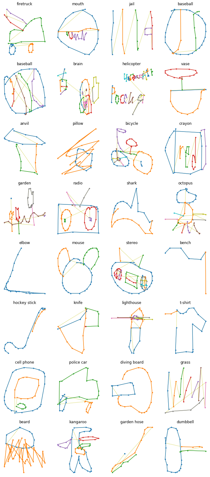
def draw_sketch(sketch, label=None):
    origin = np.array([[0., 0., 0.]])
    sketch = np.r_[origin, sketch]
    stroke_end_indices = np.argwhere(sketch[:, -1]==1.)[:, 0]
    coordinates = np.cumsum(sketch[:, :2], axis=0)
    strokes = np.split(coordinates, stroke_end_indices + 1)
    title = class_names[label.numpy()] if label is not None else "Try to guess"
    plt.title(title)
    plt.plot(coordinates[:, 0], -coordinates[:, 1], "y:")
    for stroke in strokes:
        plt.plot(stroke[:, 0], -stroke[:, 1], ".-")
    plt.axis("off")

def draw_sketches(sketches, lengths, labels):
    n_sketches = len(sketches)
    n_cols = 4
    n_rows = (n_sketches - 1) // n_cols + 1
    plt.figure(figsize=(n_cols * 3, n_rows * 3.5))
    for index, sketch, length, label in zip(range(n_sketches), sketches, lengths, labels):
        plt.subplot(n_rows, n_cols, index + 1)
        draw_sketch(sketch[:length], label)
    plt.show()

for sketches, lengths, labels in train_set.take(1):
    draw_sketches(sketches, lengths, labels)
Most sketches are composed of less than 100 points:
lengths = np.concatenate([lengths for _, lengths, _ in train_set.take(1000)])
plt.hist(lengths, bins=150, density=True)
plt.axis([0, 200, 0, 0.03])
plt.xlabel("length")
plt.ylabel("density")
plt.show()
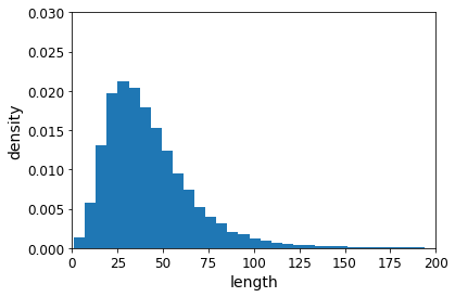
def crop_long_sketches(dataset, max_length=100):
    return dataset.map(lambda inks, lengths, labels: (inks[:, :max_length], labels))

cropped_train_set = crop_long_sketches(train_set)
cropped_valid_set = crop_long_sketches(valid_set)
cropped_test_set = crop_long_sketches(test_set)
model = keras.models.Sequential([
    keras.layers.Conv1D(32, kernel_size=5, strides=2, activation="relu"),
    keras.layers.BatchNormalization(),
    keras.layers.Conv1D(64, kernel_size=5, strides=2, activation="relu"),
    keras.layers.BatchNormalization(),
    keras.layers.Conv1D(128, kernel_size=3, strides=2, activation="relu"),
    keras.layers.BatchNormalization(),
    keras.layers.LSTM(128, return_sequences=True),
    keras.layers.LSTM(128),
    keras.layers.Dense(len(class_names), activation="softmax")
])
optimizer = keras.optimizers.SGD(learning_rate=1e-2, clipnorm=1.)
model.compile(loss="sparse_categorical_crossentropy",
              optimizer=optimizer,
              metrics=["accuracy", "sparse_top_k_categorical_accuracy"])
history = model.fit(cropped_train_set, epochs=2,
                    validation_data=cropped_valid_set)
Epoch 1/2
107813/107813 [==============================] - 2182s 20ms/step - loss: 3.8473 - accuracy: 0.2086 - sparse_top_k_categorical_accuracy: 0.4242 - val_loss: 2.6672 - val_accuracy: 0.3872 - val_sparse_top_k_categorical_accuracy: 0.6771
Epoch 2/2
107813/107813 [==============================] - 2049s 19ms/step - loss: 2.3393 - accuracy: 0.4502 - sparse_top_k_categorical_accuracy: 0.7367 - val_loss: 2.1072 - val_accuracy: 0.4968 - val_sparse_top_k_categorical_accuracy: 0.7759
y_test = np.concatenate([labels for _, _, labels in test_set])
y_probas = model.predict(test_set)
np.mean(keras.metrics.sparse_top_k_categorical_accuracy(y_test, y_probas))
0.6899671
n_new = 10
Y_probas = model.predict(sketches)
top_k = tf.nn.top_k(Y_probas, k=5)
for index in range(n_new):
    plt.figure(figsize=(3, 3.5))
    draw_sketch(sketches[index])
    plt.show()
    print("Top-5 predictions:".format(index + 1))
    for k in range(5):
        class_name = class_names[top_k.indices[index, k]]
        proba = 100 * top_k.values[index, k]
        print("  {}. {} {:.3f}%".format(k + 1, class_name, proba))
    print("Answer: {}".format(class_names[labels[index].numpy()]))
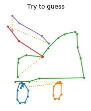
Top-5 predictions:
  1. firetruck 46.565%
  2. police car 30.455%
  3. ambulance 3.810%
  4. car 3.695%
  5. cannon 3.371%
Answer: firetruck
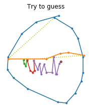
Top-5 predictions:
  1. mouth 23.162%
  2. pond 14.151%
  3. pool 12.582%
  4. beard 11.375%
  5. goatee 9.808%
Answer: mouth
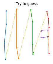
Top-5 predictions:
  1. jail 71.532%
  2. fence 6.519%
  3. swing set 5.708%
  4. grass 3.302%
  5. rain 3.023%
Answer: jail
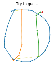
Top-5 predictions:
  1. baseball 79.233%
  2. watermelon 7.687%
  3. basketball 5.259%
  4. clock 1.659%
  5. compass 1.101%
Answer: baseball
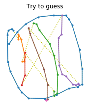
Top-5 predictions:
  1. basketball 51.888%
  2. baseball 17.328%
  3. onion 12.688%
  4. watermelon 9.989%
  5. brain 2.216%
Answer: baseball
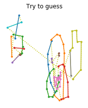
Top-5 predictions:
  1. lantern 7.235%
  2. toothpaste 6.845%
  3. drill 6.254%
  4. lighthouse 4.624%
  5. crayon 3.566%
Answer: brain
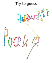
Top-5 predictions:
  1. animal migration 8.771%
  2. blackberry 7.932%
  3. blueberry 6.413%
  4. peas 5.549%
  5. bracelet 3.623%
Answer: helicopter
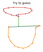
Top-5 predictions:
  1. vase 42.793%
  2. wine glass 13.744%
  3. shovel 8.136%
  4. house plant 5.144%
  5. sailboat 4.850%
Answer: vase
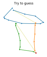
Top-5 predictions:
  1. anvil 25.870%
  2. drill 9.670%
  3. nail 7.246%
  4. screwdriver 5.611%
  5. knee 4.355%
Answer: anvil
Top-5 predictions:
  1. hurricane 34.674%
  2. tornado 16.056%
  3. blackberry 7.664%
  4. squiggle 5.489%
  5. zigzag 4.906%
Answer: pillow
model.save("my_sketchrnn")
WARNING:tensorflow:From /Users/ageron/miniconda3/envs/tf2/lib/python3.7/site-packages/tensorflow_core/python/ops/resource_variable_ops.py:1786: calling BaseResourceVariable.__init__ (from tensorflow.python.ops.resource_variable_ops) with constraint is deprecated and will be removed in a future version.
Instructions for updating:
If using Keras pass *_constraint arguments to layers.
INFO:tensorflow:Assets written to: my_sketchrnn/assets
10. Bach Chorales#
Exercise: Download the Bach chorales dataset and unzip it. It is composed of 382 chorales composed by Johann Sebastian Bach. Each chorale is 100 to 640 time steps long, and each time step contains 4 integers, where each integer corresponds to a note’s index on a piano (except for the value 0, which means that no note is played). Train a model—recurrent, convolutional, or both—that can predict the next time step (four notes), given a sequence of time steps from a chorale. Then use this model to generate Bach-like music, one note at a time: you can do this by giving the model the start of a chorale and asking it to predict the next time step, then appending these time steps to the input sequence and asking the model for the next note, and so on. Also make sure to check out Google’s Coconet model, which was used for a nice Google doodle about Bach.
DOWNLOAD_ROOT = "https://github.com/ageron/handson-ml2/raw/master/datasets/jsb_chorales/"
FILENAME = "jsb_chorales.tgz"
filepath = keras.utils.get_file(FILENAME,
                                DOWNLOAD_ROOT + FILENAME,
                                cache_subdir="datasets/jsb_chorales",
                                extract=True)
jsb_chorales_dir = Path(filepath).parent
train_files = sorted(jsb_chorales_dir.glob("train/chorale_*.csv"))
valid_files = sorted(jsb_chorales_dir.glob("valid/chorale_*.csv"))
test_files = sorted(jsb_chorales_dir.glob("test/chorale_*.csv"))
import pandas as pd

def load_chorales(filepaths):
    return [pd.read_csv(filepath).values.tolist() for filepath in filepaths]

train_chorales = load_chorales(train_files)
valid_chorales = load_chorales(valid_files)
test_chorales = load_chorales(test_files)
train_chorales[0]
[[74, 70, 65, 58],
 [74, 70, 65, 58],
 [74, 70, 65, 58],
 [74, 70, 65, 58],
 [75, 70, 58, 55],
 [75, 70, 58, 55],
 [75, 70, 60, 55],
 [75, 70, 60, 55],
 [77, 69, 62, 50],
 [77, 69, 62, 50],
 [77, 69, 62, 50],
 [77, 69, 62, 50],
 [77, 70, 62, 55],
 [77, 70, 62, 55],
 [77, 69, 62, 55],
 [77, 69, 62, 55],
 [75, 67, 63, 48],
 [75, 67, 63, 48],
 [75, 69, 63, 48],
 [75, 69, 63, 48],
 [74, 70, 65, 46],
 [74, 70, 65, 46],
 [74, 70, 65, 46],
 [74, 70, 65, 46],
 [72, 69, 65, 53],
 [72, 69, 65, 53],
 [72, 69, 65, 53],
 [72, 69, 65, 53],
 [72, 69, 65, 53],
 [72, 69, 65, 53],
 [72, 69, 65, 53],
 [72, 69, 65, 53],
 [74, 70, 65, 46],
 [74, 70, 65, 46],
 [74, 70, 65, 46],
 [74, 70, 65, 46],
 [75, 69, 63, 48],
 [75, 69, 63, 48],
 [75, 67, 63, 48],
 [75, 67, 63, 48],
 [77, 65, 62, 50],
 [77, 65, 62, 50],
 [77, 65, 60, 50],
 [77, 65, 60, 50],
 [74, 67, 58, 55],
 [74, 67, 58, 55],
 [74, 67, 58, 53],
 [74, 67, 58, 53],
 [72, 67, 58, 51],
 [72, 67, 58, 51],
 [72, 67, 58, 51],
 [72, 67, 58, 51],
 [72, 65, 57, 53],
 [72, 65, 57, 53],
 [72, 65, 57, 53],
 [72, 65, 57, 53],
 [70, 65, 62, 46],
 [70, 65, 62, 46],
 [70, 65, 62, 46],
 [70, 65, 62, 46],
 [70, 65, 62, 46],
 [70, 65, 62, 46],
 [70, 65, 62, 46],
 [70, 65, 62, 46],
 [72, 69, 65, 53],
 [72, 69, 65, 53],
 [72, 69, 65, 53],
 [72, 69, 65, 53],
 [74, 71, 53, 50],
 [74, 71, 53, 50],
 [74, 71, 53, 50],
 [74, 71, 53, 50],
 [75, 72, 55, 48],
 [75, 72, 55, 48],
 [75, 72, 55, 50],
 [75, 72, 55, 50],
 [75, 67, 60, 51],
 [75, 67, 60, 51],
 [75, 67, 60, 53],
 [75, 67, 60, 53],
 [74, 67, 60, 55],
 [74, 67, 60, 55],
 [74, 67, 57, 55],
 [74, 67, 57, 55],
 [74, 65, 59, 43],
 [74, 65, 59, 43],
 [72, 63, 59, 43],
 [72, 63, 59, 43],
 [72, 63, 55, 48],
 [72, 63, 55, 48],
 [72, 63, 55, 48],
 [72, 63, 55, 48],
 [72, 63, 55, 48],
 [72, 63, 55, 48],
 [72, 63, 55, 48],
 [72, 63, 55, 48],
 [75, 67, 60, 60],
 [75, 67, 60, 60],
 [75, 67, 60, 60],
 [75, 67, 60, 60],
 [77, 70, 62, 58],
 [77, 70, 62, 58],
 [77, 70, 62, 56],
 [77, 70, 62, 56],
 [79, 70, 62, 55],
 [79, 70, 62, 55],
 [79, 70, 62, 53],
 [79, 70, 62, 53],
 [79, 70, 63, 51],
 [79, 70, 63, 51],
 [79, 70, 63, 51],
 [79, 70, 63, 51],
 [77, 70, 63, 58],
 [77, 70, 63, 58],
 [77, 70, 60, 58],
 [77, 70, 60, 58],
 [77, 70, 62, 46],
 [77, 70, 62, 46],
 [77, 68, 62, 46],
 [75, 68, 62, 46],
 [75, 67, 58, 51],
 [75, 67, 58, 51],
 [75, 67, 58, 51],
 [75, 67, 58, 51],
 [75, 67, 58, 51],
 [75, 67, 58, 51],
 [75, 67, 58, 51],
 [75, 67, 58, 51],
 [74, 67, 58, 55],
 [74, 67, 58, 55],
 [74, 67, 58, 55],
 [74, 67, 58, 55],
 [75, 67, 58, 53],
 [75, 67, 58, 53],
 [75, 67, 58, 51],
 [75, 67, 58, 51],
 [77, 65, 58, 50],
 [77, 65, 58, 50],
 [77, 65, 56, 50],
 [77, 65, 56, 50],
 [70, 63, 55, 51],
 [70, 63, 55, 51],
 [70, 63, 55, 51],
 [70, 63, 55, 51],
 [75, 65, 60, 45],
 [75, 65, 60, 45],
 [75, 65, 60, 45],
 [75, 65, 60, 45],
 [74, 65, 58, 46],
 [74, 65, 58, 46],
 [74, 65, 58, 46],
 [74, 65, 58, 46],
 [72, 65, 57, 53],
 [72, 65, 57, 53],
 [72, 65, 57, 53],
 [72, 65, 57, 53],
 [72, 65, 57, 53],
 [72, 65, 57, 53],
 [72, 65, 57, 53],
 [72, 65, 57, 53],
 [74, 65, 58, 58],
 [74, 65, 58, 58],
 [74, 65, 58, 58],
 [74, 65, 58, 58],
 [75, 67, 58, 57],
 [75, 67, 58, 57],
 [75, 67, 58, 55],
 [75, 67, 58, 55],
 [77, 65, 60, 57],
 [77, 65, 60, 57],
 [77, 65, 60, 53],
 [77, 65, 60, 53],
 [74, 65, 58, 58],
 [74, 65, 58, 58],
 [74, 65, 58, 58],
 [74, 65, 58, 58],
 [72, 67, 58, 51],
 [72, 67, 58, 51],
 [72, 67, 58, 51],
 [72, 67, 58, 51],
 [72, 65, 57, 53],
 [72, 65, 57, 53],
 [72, 65, 57, 53],
 [72, 65, 57, 53],
 [70, 65, 62, 46],
 [70, 65, 62, 46],
 [70, 65, 62, 46],
 [70, 65, 62, 46],
 [70, 65, 62, 46],
 [70, 65, 62, 46],
 [70, 65, 62, 46],
 [70, 65, 62, 46]]
Notes range from 36 (C1 = C on octave 1) to 81 (A5 = A on octave 5), plus 0 for silence:
notes = set()
for chorales in (train_chorales, valid_chorales, test_chorales):
    for chorale in chorales:
        for chord in chorale:
            notes |= set(chord)

n_notes = len(notes)
min_note = min(notes - {0})
max_note = max(notes)

assert min_note == 36
assert max_note == 81
Let’s write a few functions to listen to these chorales (you don’t need to understand the details here, and in fact there are certainly simpler ways to do this, for example using MIDI players, but I just wanted to have a bit of fun writing a synthesizer):
from IPython.display import Audio

def notes_to_frequencies(notes):
    # Frequency doubles when you go up one octave; there are 12 semi-tones
    # per octave; Note A on octave 4 is 440 Hz, and it is note number 69.
    return 2 ** ((np.array(notes) - 69) / 12) * 440

def frequencies_to_samples(frequencies, tempo, sample_rate):
    note_duration = 60 / tempo # the tempo is measured in beats per minutes
    # To reduce click sound at every beat, we round the frequencies to try to
    # get the samples close to zero at the end of each note.
    frequencies = np.round(note_duration * frequencies) / note_duration
    n_samples = int(note_duration * sample_rate)
    time = np.linspace(0, note_duration, n_samples)
    sine_waves = np.sin(2 * np.pi * frequencies.reshape(-1, 1) * time)
    # Removing all notes with frequencies ≤ 9 Hz (includes note 0 = silence)
    sine_waves *= (frequencies > 9.).reshape(-1, 1)
    return sine_waves.reshape(-1)

def chords_to_samples(chords, tempo, sample_rate):
    freqs = notes_to_frequencies(chords)
    freqs = np.r_[freqs, freqs[-1:]] # make last note a bit longer
    merged = np.mean([frequencies_to_samples(melody, tempo, sample_rate)
                     for melody in freqs.T], axis=0)
    n_fade_out_samples = sample_rate * 60 // tempo # fade out last note
    fade_out = np.linspace(1., 0., n_fade_out_samples)**2
    merged[-n_fade_out_samples:] *= fade_out
    return merged

def play_chords(chords, tempo=160, amplitude=0.1, sample_rate=44100, filepath=None):
    samples = amplitude * chords_to_samples(chords, tempo, sample_rate)
    if filepath:
        from scipy.io import wavfile
        samples = (2**15 * samples).astype(np.int16)
        wavfile.write(filepath, sample_rate, samples)
        return display(Audio(filepath))
    else:
        return display(Audio(samples, rate=sample_rate))
Now let’s listen to a few chorales:
for index in range(3):
    play_chords(train_chorales[index])
Divine! :)
In order to be able to generate new chorales, we want to train a model that can predict the next chord given all the previous chords. If we naively try to predict the next chord in one shot, predicting all 4 notes at once, we run the risk of getting notes that don’t go very well together (believe me, I tried). It’s much better and simpler to predict one note at a time. So we will need to preprocess every chorale, turning each chord into an arpegio (i.e., a sequence of notes rather than notes played simultaneuously). So each chorale will be a long sequence of notes (rather than chords), and we can just train a model that can predict the next note given all the previous notes. We will use a sequence-to-sequence approach, where we feed a window to the neural net, and it tries to predict that same window shifted one time step into the future.
We will also shift the values so that they range from 0 to 46, where 0 represents silence, and values 1 to 46 represent notes 36 (C1) to 81 (A5).
And we will train the model on windows of 128 notes (i.e., 32 chords).
Since the dataset fits in memory, we could preprocess the chorales in RAM using any Python code we like, but I will demonstrate here how to do all the preprocessing using tf.data (there will be more details about creating windows using tf.data in the next chapter).
def create_target(batch):
    X = batch[:, :-1]
    Y = batch[:, 1:] # predict next note in each arpegio, at each step
    return X, Y

def preprocess(window):
    window = tf.where(window == 0, window, window - min_note + 1) # shift values
    return tf.reshape(window, [-1]) # convert to arpegio

def bach_dataset(chorales, batch_size=32, shuffle_buffer_size=None,
                 window_size=32, window_shift=16, cache=True):
    def batch_window(window):
        return window.batch(window_size + 1)

    def to_windows(chorale):
        dataset = tf.data.Dataset.from_tensor_slices(chorale)
        dataset = dataset.window(window_size + 1, window_shift, drop_remainder=True)
        return dataset.flat_map(batch_window)

    chorales = tf.ragged.constant(chorales, ragged_rank=1)
    dataset = tf.data.Dataset.from_tensor_slices(chorales)
    dataset = dataset.flat_map(to_windows).map(preprocess)
    if cache:
        dataset = dataset.cache()
    if shuffle_buffer_size:
        dataset = dataset.shuffle(shuffle_buffer_size)
    dataset = dataset.batch(batch_size)
    dataset = dataset.map(create_target)
    return dataset.prefetch(1)
Now let’s create the training set, the validation set and the test set:
train_set = bach_dataset(train_chorales, shuffle_buffer_size=1000)
valid_set = bach_dataset(valid_chorales)
test_set = bach_dataset(test_chorales)
Now let’s create the model:
We could feed the note values directly to the model, as floats, but this would probably not give good results. Indeed, the relationships between notes are not that simple: for example, if you replace a C3 with a C4, the melody will still sound fine, even though these notes are 12 semi-tones apart (i.e., one octave). Conversely, if you replace a C3 with a C#3, it’s very likely that the chord will sound horrible, despite these notes being just next to each other. So we will use an
Embeddinglayer to convert each note to a small vector representation (see Chapter 16 for more details on embeddings). We will use 5-dimensional embeddings, so the output of this first layer will have a shape of[batch_size, window_size, 5].We will then feed this data to a small WaveNet-like neural network, composed of a stack of 4
Conv1Dlayers with doubling dilation rates. We will intersperse these layers withBatchNormalizationlayers for faster better convergence.Then one
LSTMlayer to try to capture long-term patterns.And finally a
Denselayer to produce the final note probabilities. It will predict one probability for each chorale in the batch, for each time step, and for each possible note (including silence). So the output shape will be[batch_size, window_size, 47].
n_embedding_dims = 5

model = keras.models.Sequential([
    keras.layers.Embedding(input_dim=n_notes, output_dim=n_embedding_dims,
                           input_shape=[None]),
    keras.layers.Conv1D(32, kernel_size=2, padding="causal", activation="relu"),
    keras.layers.BatchNormalization(),
    keras.layers.Conv1D(48, kernel_size=2, padding="causal", activation="relu", dilation_rate=2),
    keras.layers.BatchNormalization(),
    keras.layers.Conv1D(64, kernel_size=2, padding="causal", activation="relu", dilation_rate=4),
    keras.layers.BatchNormalization(),
    keras.layers.Conv1D(96, kernel_size=2, padding="causal", activation="relu", dilation_rate=8),
    keras.layers.BatchNormalization(),
    keras.layers.LSTM(256, return_sequences=True),
    keras.layers.Dense(n_notes, activation="softmax")
])

model.summary()
Model: "sequential"
_________________________________________________________________
Layer (type)                 Output Shape              Param #
=================================================================
embedding (Embedding)        (None, None, 5)           235
_________________________________________________________________
conv1d (Conv1D)              (None, None, 32)          352
_________________________________________________________________
batch_normalization (BatchNo (None, None, 32)          128
_________________________________________________________________
conv1d_1 (Conv1D)            (None, None, 48)          3120
_________________________________________________________________
batch_normalization_1 (Batch (None, None, 48)          192
_________________________________________________________________
conv1d_2 (Conv1D)            (None, None, 64)          6208
_________________________________________________________________
batch_normalization_2 (Batch (None, None, 64)          256
_________________________________________________________________
conv1d_3 (Conv1D)            (None, None, 96)          12384
_________________________________________________________________
batch_normalization_3 (Batch (None, None, 96)          384
_________________________________________________________________
lstm (LSTM)                  (None, None, 256)         361472
_________________________________________________________________
dense (Dense)                (None, None, 47)          12079
=================================================================
Total params: 396,810
Trainable params: 396,330
Non-trainable params: 480
_________________________________________________________________
Now we’re ready to compile and train the model!
optimizer = keras.optimizers.Nadam(learning_rate=1e-3)
model.compile(loss="sparse_categorical_crossentropy", optimizer=optimizer,
              metrics=["accuracy"])
model.fit(train_set, epochs=20, validation_data=valid_set)
Epoch 1/20
98/98 [==============================] - 17s 171ms/step - loss: 1.8198 - accuracy: 0.5358 - val_loss: 3.7675 - val_accuracy: 0.0428
Epoch 2/20
98/98 [==============================] - 15s 152ms/step - loss: 0.8885 - accuracy: 0.7641 - val_loss: 4.1054 - val_accuracy: 0.0470
Epoch 3/20
98/98 [==============================] - 16s 165ms/step - loss: 0.7471 - accuracy: 0.7930 - val_loss: 3.8600 - val_accuracy: 0.0368
Epoch 4/20
98/98 [==============================] - 16s 165ms/step - loss: 0.6749 - accuracy: 0.8083 - val_loss: 3.0490 - val_accuracy: 0.2196
Epoch 5/20
98/98 [==============================] - 15s 157ms/step - loss: 0.6221 - accuracy: 0.8188 - val_loss: 1.7138 - val_accuracy: 0.5153
Epoch 6/20
98/98 [==============================] - 16s 163ms/step - loss: 0.5833 - accuracy: 0.8283 - val_loss: 1.9068 - val_accuracy: 0.4570
Epoch 7/20
98/98 [==============================] - 16s 165ms/step - loss: 0.5484 - accuracy: 0.8362 - val_loss: 0.7930 - val_accuracy: 0.7678
Epoch 8/20
98/98 [==============================] - 16s 159ms/step - loss: 0.5163 - accuracy: 0.8447 - val_loss: 0.6577 - val_accuracy: 0.8091
Epoch 9/20
98/98 [==============================] - 15s 158ms/step - loss: 0.4877 - accuracy: 0.8519 - val_loss: 0.6239 - val_accuracy: 0.8180
Epoch 10/20
98/98 [==============================] - 17s 171ms/step - loss: 0.4607 - accuracy: 0.8595 - val_loss: 0.6330 - val_accuracy: 0.8151
Epoch 11/20
98/98 [==============================] - 15s 156ms/step - loss: 0.4369 - accuracy: 0.8657 - val_loss: 0.6248 - val_accuracy: 0.8179
Epoch 12/20
98/98 [==============================] - 16s 167ms/step - loss: 0.4125 - accuracy: 0.8726 - val_loss: 0.6046 - val_accuracy: 0.8248
Epoch 13/20
98/98 [==============================] - 16s 162ms/step - loss: 0.3924 - accuracy: 0.8784 - val_loss: 0.6618 - val_accuracy: 0.8096
Epoch 14/20
98/98 [==============================] - 16s 159ms/step - loss: 0.3713 - accuracy: 0.8847 - val_loss: 0.6919 - val_accuracy: 0.8067
Epoch 15/20
98/98 [==============================] - 17s 176ms/step - loss: 0.3562 - accuracy: 0.8889 - val_loss: 0.6123 - val_accuracy: 0.8236
Epoch 16/20
98/98 [==============================] - 16s 165ms/step - loss: 0.3328 - accuracy: 0.8969 - val_loss: 0.6547 - val_accuracy: 0.8133
Epoch 17/20
98/98 [==============================] - 15s 156ms/step - loss: 0.3182 - accuracy: 0.9011 - val_loss: 0.6322 - val_accuracy: 0.8202
Epoch 18/20
98/98 [==============================] - 16s 167ms/step - loss: 0.3007 - accuracy: 0.9069 - val_loss: 0.6929 - val_accuracy: 0.8037
Epoch 19/20
98/98 [==============================] - 16s 168ms/step - loss: 0.2869 - accuracy: 0.9103 - val_loss: 0.6446 - val_accuracy: 0.8220
Epoch 20/20
98/98 [==============================] - 17s 173ms/step - loss: 0.2703 - accuracy: 0.9158 - val_loss: 0.6439 - val_accuracy: 0.8189
<tensorflow.python.keras.callbacks.History at 0x7fee205ff490>
I have not done much hyperparameter search, so feel free to iterate on this model now and try to optimize it. For example, you could try removing the LSTM layer and replacing it with Conv1D layers. You could also play with the number of layers, the learning rate, the optimizer, and so on.
Once you’re satisfied with the performance of the model on the validation set, you can save it and evaluate it one last time on the test set:
model.save("my_bach_model.h5")
model.evaluate(test_set)
34/Unknown - 2s 66ms/step - loss: 0.6557 - accuracy: 0.8164
[0.6556663916391485, 0.8164004]
Note: There’s no real need for a test set in this exercise, since we will perform the final evaluation by just listening to the music produced by the model. So if you want, you can add the test set to the train set, and train the model again, hopefully getting a slightly better model.
Now let’s write a function that will generate a new chorale. We will give it a few seed chords, it will convert them to arpegios (the format expected by the model), and use the model to predict the next note, then the next, and so on. In the end, it will group the notes 4 by 4 to create chords again, and return the resulting chorale.
Warning: model.predict_classes(X) is deprecated. It is replaced with np.argmax(model.predict(X), axis=-1).
def generate_chorale(model, seed_chords, length):
    arpegio = preprocess(tf.constant(seed_chords, dtype=tf.int64))
    arpegio = tf.reshape(arpegio, [1, -1])
    for chord in range(length):
        for note in range(4):
            #next_note = model.predict_classes(arpegio)[:1, -1:]
            next_note = np.argmax(model.predict(arpegio), axis=-1)[:1, -1:]
            arpegio = tf.concat([arpegio, next_note], axis=1)
    arpegio = tf.where(arpegio == 0, arpegio, arpegio + min_note - 1)
    return tf.reshape(arpegio, shape=[-1, 4])
To test this function, we need some seed chords. Let’s use the first 8 chords of one of the test chorales (it’s actually just 2 different chords, each played 4 times):
seed_chords = test_chorales[2][:8]
play_chords(seed_chords, amplitude=0.2)
Now we are ready to generate our first chorale! Let’s ask the function to generate 56 more chords, for a total of 64 chords, i.e., 16 bars (assuming 4 chords per bar, i.e., a 4/4 signature):
new_chorale = generate_chorale(model, seed_chords, 56)
play_chords(new_chorale)
This approach has one major flaw: it is often too conservative. Indeed, the model will not take any risk, it will always choose the note with the highest score, and since repeating the previous note generally sounds good enough, it’s the least risky option, so the algorithm will tend to make notes last longer and longer. Pretty boring. Plus, if you run the model multiple times, it will always generate the same melody.
So let’s spice things up a bit! Instead of always picking the note with the highest score, we will pick the next note randomly, according to the predicted probabilities. For example, if the model predicts a C3 with 75% probability, and a G3 with a 25% probability, then we will pick one of these two notes randomly, with these probabilities. We will also add a temperature parameter that will control how “hot” (i.e., daring) we want the system to feel. A high temperature will bring the predicted probabilities closer together, reducing the probability of the likely notes and increasing the probability of the unlikely ones.
def generate_chorale_v2(model, seed_chords, length, temperature=1):
    arpegio = preprocess(tf.constant(seed_chords, dtype=tf.int64))
    arpegio = tf.reshape(arpegio, [1, -1])
    for chord in range(length):
        for note in range(4):
            next_note_probas = model.predict(arpegio)[0, -1:]
            rescaled_logits = tf.math.log(next_note_probas) / temperature
            next_note = tf.random.categorical(rescaled_logits, num_samples=1)
            arpegio = tf.concat([arpegio, next_note], axis=1)
    arpegio = tf.where(arpegio == 0, arpegio, arpegio + min_note - 1)
    return tf.reshape(arpegio, shape=[-1, 4])
Let’s generate 3 chorales using this new function: one cold, one medium, and one hot (feel free to experiment with other seeds, lengths and temperatures). The code saves each chorale to a separate file. You can run these cells over an over again until you generate a masterpiece!
Please share your most beautiful generated chorale with me on Twitter @aureliengeron, I would really appreciate it! :))
new_chorale_v2_cold = generate_chorale_v2(model, seed_chords, 56, temperature=0.8)
play_chords(new_chorale_v2_cold, filepath="bach_cold.wav")
new_chorale_v2_medium = generate_chorale_v2(model, seed_chords, 56, temperature=1.0)
play_chords(new_chorale_v2_medium, filepath="bach_medium.wav")
new_chorale_v2_hot = generate_chorale_v2(model, seed_chords, 56, temperature=1.5)
play_chords(new_chorale_v2_hot, filepath="bach_hot.wav")
Lastly, you can try a fun social experiment: send your friends a few of your favorite generated chorales, plus the real chorale, and ask them to guess which one is the real one!
play_chords(test_chorales[2][:64], filepath="bach_test_4.wav")