IML with Pima Indians and the Titanic datasets#
source: Parul Pandey on Kaggle

In his book ‘Interpretable Machine Learning’, Christoph Molnar beautifully encapsulates the essence of ML interpretability through this example: Imagine you are a Data Scientist and in your free time you try to predict where your friends will go on vacation in the summer based on their facebook and twitter data you have. Now, if the predictions turn out to be accurate, your friends might be impressed and could consider you to be a magician who could see the future.
If the predictions are wrong, it would still bring no harm to anyone except to your reputation of being a “Data Scientist”. Now let’s say it wasn’t a fun project and there were investments involved. Say, you wanted to invest in properties where your friends were likely to holiday. What would happen if the model’s predictions went awry?You would lose money. As long as the model is having no significant impact, it’s interpretability doesn’t matter so much but when there are implications involved based on a model’s prediction, be it financial or social, interpretability becomes relevant.
Importance of interpretability#
The question that some of the people often ask is why aren’t we just content with the results of the model and why are we so hell-bent on knowing why a particular decision was made? A lot of this has to do with the impact that a model might have in the real world. For models which are merely meant to recommend movies will have a far less impact than the ones created to predict the outcome of a drug.
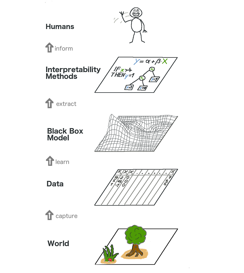
The big picture of explainable machine learning.
Some of the benefits that interpretability brings along are:

Model Explainability techniques#
Let’s discuss a few techniques which help in extracting the above insights from a model. These techniques in the order in which they are discussed are as follows:
ELI5 library
Partial Dependence Plots
SHAP Values
Advanced Uses of SHAP Values
SHAP Summary Plots
LIME
SHAP Values
Advanced Uses of SHAP Values
SHAP Summary Plots
LIME
SHAP Summary Plots
LIME
Objective#
The objective of the notebook is to use techniques to explain how different features have different effect on the prediction whether or not a patient has diabetes, based on certain diagnostic measurements.
# Loading necessary libraries

import numpy as np # linear algebra
import pandas as pd # data processing, CSV file I/O (e.g. pd.read_csv)
from sklearn.model_selection import train_test_split
from sklearn.ensemble import RandomForestClassifier
from sklearn.model_selection import train_test_split
from matplotlib import pyplot as plt
%matplotlib inline

from sklearn.preprocessing import LabelEncoder
import lightgbm as lgb
# Reading in the data
df = pd.read_csv('./data/diabetes.csv')
df.head()
| Pregnancies | Glucose | BloodPressure | SkinThickness | Insulin | BMI | DiabetesPedigreeFunction | Age | Outcome | |
|---|---|---|---|---|---|---|---|---|---|
| 0 | 6 | 148 | 72 | 35 | 0 | 33.6 | 0.627 | 50 | 1 |
| 1 | 1 | 85 | 66 | 29 | 0 | 26.6 | 0.351 | 31 | 0 |
| 2 | 8 | 183 | 64 | 0 | 0 | 23.3 | 0.672 | 32 | 1 |
| 3 | 1 | 89 | 66 | 23 | 94 | 28.1 | 0.167 | 21 | 0 |
| 4 | 0 | 137 | 40 | 35 | 168 | 43.1 | 2.288 | 33 | 1 |
df.info()
<class 'pandas.core.frame.DataFrame'>
RangeIndex: 768 entries, 0 to 767
Data columns (total 9 columns):
 #   Column                    Non-Null Count  Dtype
---  ------                    --------------  -----
 0   Pregnancies               768 non-null    int64
 1   Glucose                   768 non-null    int64
 2   BloodPressure             768 non-null    int64
 3   SkinThickness             768 non-null    int64
 4   Insulin                   768 non-null    int64
 5   BMI                       768 non-null    float64
 6   DiabetesPedigreeFunction  768 non-null    float64
 7   Age                       768 non-null    int64
 8   Outcome                   768 non-null    int64
dtypes: float64(2), int64(7)
memory usage: 54.1 KB
# Creating the target and the features column and splitting the dataset into test and train set.

X = df.iloc[:, :-1]
y = df.iloc[:, -1]

X_train, X_test, y_train, y_test = train_test_split(X, y, test_size=0.25, random_state=0)
1. Permutation Importance using ELI5 library#
What features does a model think are important? Which features might have a greater impact on the model predictions than the others? This concept is called feature importance and Permutation Importance is a technique used widely for calculating feature importance. It helps us to see when our model produces counterintuitive results, and it helps to show the others when our model is working as we’d hope.
Permutation Importance works for many scikit-learn estimators. The idea is simple: Randomly permutate or shuffle a single column in the validation dataset leaving all the other columns intact. A feature is considered “important” if the model’s accuracy drops a lot and causes an increase in error. On the other hand, a feature is considered ‘unimportant’ if shuffling its values don’t affect the model’s accuracy.
Permutation importance is useful useful for debugging, understanding your model, and communicating a high-level overview from your model.
Permutation importance is calculated after a model has been fitted. So, let’s train and fit a RandomForestClassifier model denoted as my_model on the training data.
Permutation Importance is calculated using the ELI5 library. ELI5 is a Python library which allows to visualize and debug various Machine Learning models using unified API. It has built-in support for several ML frameworks and provides a way to explain black-box models.
# Training and fitting a Random Forest Model
my_model = RandomForestClassifier(n_estimators=100,
                                  random_state=0).fit(X_train, y_train)
# Calculating and Displaying importance using the eli5 library
import eli5
from eli5.sklearn import PermutationImportance

perm = PermutationImportance(my_model, random_state=1).fit(X_test,y_test)
eli5.show_weights(perm, feature_names = X_test.columns.tolist())
---------------------------------------------------------------------------
ImportError                               Traceback (most recent call last)
Cell In[6], line 2
      1 # Calculating and Displaying importance using the eli5 library
----> 2 import eli5
      3 from eli5.sklearn import PermutationImportance
      5 perm = PermutationImportance(my_model, random_state=1).fit(X_test,y_test)

File /opt/hostedtoolcache/Python/3.8.18/x64/lib/python3.8/site-packages/eli5/__init__.py:13
      6 from .formatters import (
      7     format_as_html,
      8     format_html_styles,
      9     format_as_text,
     10     format_as_dict,
     11 )
     12 from .explain import explain_weights, explain_prediction
---> 13 from .sklearn import explain_weights_sklearn, explain_prediction_sklearn
     14 from .transform import transform_feature_names
     17 try:

File /opt/hostedtoolcache/Python/3.8.18/x64/lib/python3.8/site-packages/eli5/sklearn/__init__.py:3
      1 # -*- coding: utf-8 -*-
      2 from __future__ import absolute_import
----> 3 from .explain_weights import (
      4     explain_weights_sklearn,
      5     explain_linear_classifier_weights,
      6     explain_linear_regressor_weights,
      7     explain_rf_feature_importance,
      8     explain_decision_tree,
      9 )
     10 from .explain_prediction import (
     11     explain_prediction_sklearn,
     12     explain_prediction_linear_classifier,
     13     explain_prediction_linear_regressor,
     14 )
     15 from .unhashing import (
     16     InvertableHashingVectorizer,
     17     FeatureUnhasher,
     18     invert_hashing_and_fit,
     19 )

File /opt/hostedtoolcache/Python/3.8.18/x64/lib/python3.8/site-packages/eli5/sklearn/explain_weights.py:78
     73 from eli5.transform import transform_feature_names
     74 from eli5._feature_importances import (
     75     get_feature_importances_filtered,
     76     get_feature_importance_explanation,
     77 )
---> 78 from .permutation_importance import PermutationImportance
     81 LINEAR_CAVEATS = """
     82 Caveats:
     83 1. Be careful with features which are not
   (...)
     90    classification result for most examples.
     91 """.lstrip()
     93 HASHING_CAVEATS = """
     94 Feature names are restored from their hashes; this is not 100% precise
     95 because collisions are possible. For known collisions possible feature names
   (...)
     99 the result is positive.
    100 """.lstrip()

File /opt/hostedtoolcache/Python/3.8.18/x64/lib/python3.8/site-packages/eli5/sklearn/permutation_importance.py:7
      5 import numpy as np
      6 from sklearn.model_selection import check_cv
----> 7 from sklearn.utils.metaestimators import if_delegate_has_method
      8 from sklearn.utils import check_array, check_random_state
      9 from sklearn.base import (
     10     BaseEstimator,
     11     MetaEstimatorMixin,
     12     clone,
     13     is_classifier
     14 )

ImportError: cannot import name 'if_delegate_has_method' from 'sklearn.utils.metaestimators' (/opt/hostedtoolcache/Python/3.8.18/x64/lib/python3.8/site-packages/sklearn/utils/metaestimators.py)
Interpretation
The features at the top are most important and at the bottom, the least. For this example, ‘Glucose level’ is the most important feature which decides whether a person will have diabetes, which also makes sense.
The number after the ± measures how performance varied from one-reshuffling to the next.
Some weights are negative. This is because in those cases predictions on the shuffled data were found to be more accurate than the real data.
2. Partial Dependence Plots#
The partial dependence plot (short PDP or PD plot) shows the marginal effect one or two features have on the predicted outcome of a machine learning model( J. H. Friedman 2001). PDPs show how a feature affects predictions. PDP can show the relationship between the target and the selected features via 1D or 2D plots.
# training and fitting a Decision Tree
from sklearn.tree import DecisionTreeClassifier
feature_names = [i for i in df.columns]
tree_model = DecisionTreeClassifier(random_state=0).fit(X_train, y_train)
feature_names = ['Pregnancies', 'Glucose', 'BloodPressure', 'SkinThickness', 'Insulin',
       'BMI', 'DiabetesPedigreeFunction', 'Age']
# Let's plot a decision tree source : #https://www.kaggle.com/willkoehrsen/visualize-a-decision-tree-w-python-scikit-learn
# Since there are a lot of attributes, it is difficult to actually make sense of the decision tree graph in this notebook.
# It is advised to export it as png and view it.

from sklearn import tree
import graphviz

tree_graph = tree.export_graphviz(tree_model, out_file=None, feature_names=feature_names,filled = True)
graphviz.Source(tree_graph)

The library to be used for plotting PDPs is called python partial dependence plot toolbox or simply [PDPbox]. PDPs are also calculated after a model has been fit. In our dataset there are a lot of features like Glucose, BLood Pressure, Age etc. We start by considering a single row.
We proceed by fitting our model and calculating the probability of a person having diabetes which is our target variable. Next, we would choose a variable and continuously alter its value. For instance, we will calculate the outcome if the person’s insulin level is 50,100,150 and so on. All these values are then plotted and we get a graph of predicted vs actual outcome.(https://pdpbox.readthedocs.io/en/latest/)
from pdpbox import pdp, get_dataset, info_plots

# Create the data that we will plot
pdp_goals = pdp.pdp_isolate(model=tree_model, dataset=X_test, model_features=feature_names, feature='Glucose')

# plot it
pdp.pdp_plot(pdp_goals, 'Glucose')
plt.show()
/opt/hostedtoolcache/Python/3.8.18/x64/lib/python3.8/site-packages/tqdm/auto.py:21: TqdmWarning: IProgress not found. Please update jupyter and ipywidgets. See https://ipywidgets.readthedocs.io/en/stable/user_install.html
  from .autonotebook import tqdm as notebook_tqdm
---------------------------------------------------------------------------
ImportError                               Traceback (most recent call last)
Cell In[10], line 1
----> 1 from pdpbox import pdp, get_dataset, info_plots
      3 # Create the data that we will plot
      4 pdp_goals = pdp.pdp_isolate(model=tree_model, dataset=X_test, model_features=feature_names, feature='Glucose')

ImportError: cannot import name 'get_dataset' from 'pdpbox' (/opt/hostedtoolcache/Python/3.8.18/x64/lib/python3.8/site-packages/pdpbox/__init__.py)
# Create the data that we will plot
pdp_goals = pdp.pdp_isolate(model=tree_model, dataset=X_test, model_features=feature_names, feature='Insulin')

# plot it
pdp.pdp_plot(pdp_goals, 'Insulin')
plt.show()
---------------------------------------------------------------------------
AttributeError                            Traceback (most recent call last)
Cell In[11], line 2
      1 # Create the data that we will plot
----> 2 pdp_goals = pdp.pdp_isolate(model=tree_model, dataset=X_test, model_features=feature_names, feature='Insulin')
      4 # plot it
      5 pdp.pdp_plot(pdp_goals, 'Insulin')

AttributeError: module 'pdpbox.pdp' has no attribute 'pdp_isolate'
Interpretation
The Y-axis represents the change in prediction from what it would be predicted at the baseline or leftmost value.
Blue area denotes the confidence interval
For the ‘Glucose’ graph, we observe that probability of a person having diabetes steeply increases as the glucose level goes beyond 140 and then the probability remains high.
We can also visualize the partial dependence of two features at once using 2D Partial plots.
features_to_plot = ['Glucose','Insulin']
inter1  =  pdp.pdp_interact(model=tree_model, dataset=X_test, model_features=feature_names, features=features_to_plot)

pdp.pdp_interact_plot(pdp_interact_out=inter1, feature_names=features_to_plot, plot_type='contour', plot_pdp=True)
plt.show()
---------------------------------------------------------------------------
AttributeError                            Traceback (most recent call last)
Cell In[12], line 2
      1 features_to_plot = ['Glucose','Insulin']
----> 2 inter1  =  pdp.pdp_interact(model=tree_model, dataset=X_test, model_features=feature_names, features=features_to_plot)
      4 pdp.pdp_interact_plot(pdp_interact_out=inter1, feature_names=features_to_plot, plot_type='contour', plot_pdp=True)
      5 plt.show()

AttributeError: module 'pdpbox.pdp' has no attribute 'pdp_interact'
3. SHAP Values#
SHAP which stands for SHapley Additive exPlanation, helps to break down a prediction to show the impact of each feature. It is based on Shapley values, a technique used in game theory to determine how much each player in a collaborative game has contributed to its success¹. Normally, getting the trade-off between accuracy and interpretability just right can be a difficult balancing act but SHAP values can deliver both.
SHAP values interpret the impact of having a certain value for a given feature in comparison to the prediction we’d make if that feature took some baseline value.
Shap values show how much a given feature changed our prediction (compared to if we made that prediction at some baseline value of that feature). Let’s say we wanted to know what was the prediction when the insulin level was 150 instead of some fixed baseline no. If we are able to answer this, we could perform the same steps for other features as follows:
sum(SHAP values for all features) = pred_for_team - pred_for_baseline_values
row_to_show = 10
data_for_prediction = X_test.iloc[row_to_show]  # use 1 row of data here. Could use multiple rows if desired
data_for_prediction_array = data_for_prediction.values.reshape(1, -1)

tree_model.predict_proba(data_for_prediction_array)
array([[0., 1.]])
SHAP values are calculated using the Shap library which can be installed easily from PyPI or conda. SHAP values interpret the impact of having a certain value for a given feature in comparison to the prediction we’d make if that feature took some baseline value.
import shap  # package used to calculate Shap values

# Create object that can calculate shap values
explainer = shap.TreeExplainer(tree_model)

# Calculate Shap values
shap_values = explainer.shap_values(data_for_prediction)
shap.initjs()
shap.force_plot(explainer.expected_value[1], shap_values[1], data_for_prediction)

Have you run `initjs()` in this notebook? If this notebook was from another user you must also trust this notebook (File -> Trust notebook). If you are viewing this notebook on github the Javascript has been stripped for security. If you are using JupyterLab this error is because a JupyterLab extension has not yet been written.
Interpretation
The above explanation shows features each contributing to push the model output from the base value (the average model output over the training dataset we passed) to the model output. Features pushing the prediction higher are shown in red, those pushing the prediction lower are in blue
The base_value here is 0.3576 while our predicted value is 1.
Glucose= 158 has the biggest impact on increasing the prediction, whileAgefeature has the biggest effect in decreasing the prediction.
4. Advanced Uses of SHAP Values#
Aggregating many SHAP values can provide even more detailed insights into the model.
SHAP Summary Plots
To get an overview of which features are most important for a model we can plot the SHAP values of every feature for every sample. The summary plot tells which features are most important, and also their range of effects over the dataset.
import shap  # package used to calculate Shap values

# Create object that can calculate shap values
explainer = shap.TreeExplainer(tree_model)

# calculate shap values. This is what we will plot.
# Calculate shap_values for all of val_X rather than a single row, to have more data for plot.
shap_values = explainer.shap_values(X_test)

# Make plot. Index of [1] is explained in text below.
shap.summary_plot(shap_values[1],X_test)
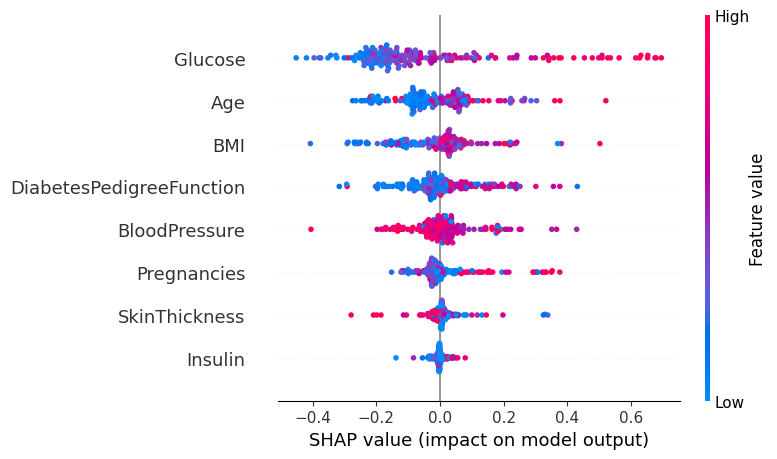
For every dot:
Vertical location shows what feature it is depicting
Color shows whether that feature was high or low for that row of the dataset
Horizontal location shows whether the effect of that value caused a higher or lower prediction.
The point in the upper left was depicts a person whose glucose level is less thereby reducing the prediction of diabetes by 0.4.
5. LIME: Locally Interpretable Model-Agnostic Explanations#
The framework LIME is introduced in a paper titled: “Why Should I Trust You?”: Explaining the Predictions of Any Classifier. This paper talks about an algorithm that is capable of explaining the predicitons of a ML model(classification/Regression problem) in a reasonable way.LIME essentially approximates the predictions of the blackbox models locally with an intrepretable model.
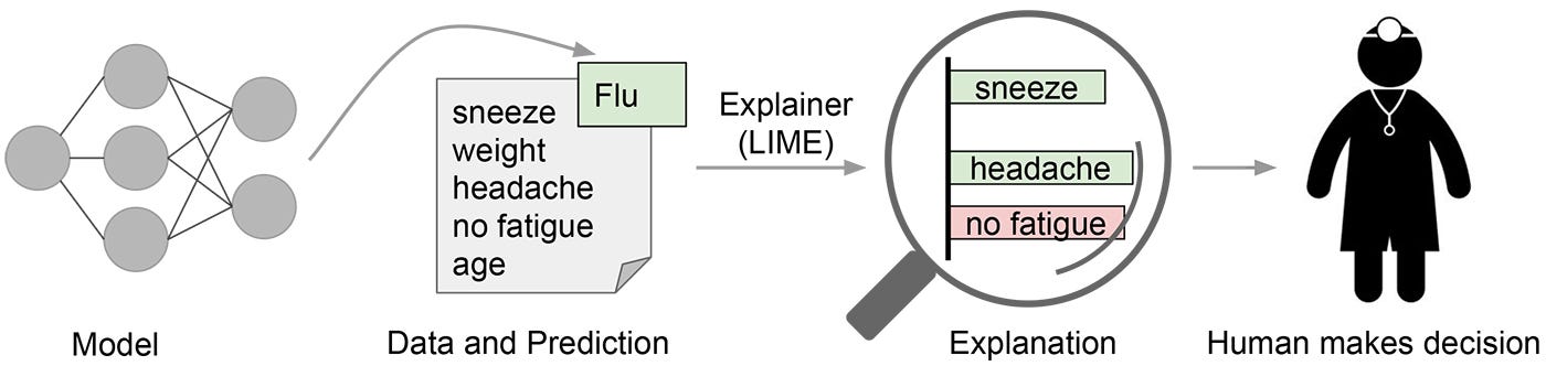 LIME attempts to play the role of the ‘explainer’, explaining predictions for each data sample. Source
To make it more understandable, I shall be using the Titanic dataset for this part of the notebook.
import lime
from lime.lime_tabular import LimeTabularExplainer

# Reading in the data
df_titanic = pd.read_csv('./data/titanic/train.csv')
df_titanic.drop('PassengerId',axis=1,inplace=True)

# Filling the missing values
df_titanic.fillna(0,inplace=True)

# label encoding categorical data
le = LabelEncoder()

df_titanic['Pclass_le'] = le.fit_transform(df_titanic['Pclass'])
df_titanic['SibSp_le'] = le.fit_transform(df_titanic['SibSp'])
df_titanic['Sex_le'] = le.fit_transform(df_titanic['Sex'])

cat_col = ['Pclass_le', 'Sex_le','SibSp_le', 'Parch','Fare']

# create validation set
X_train,X_test,y_train,y_test = train_test_split(df_titanic[cat_col],df_titanic[['Survived']],test_size=0.3)


# create dataset for lightgbm
lgb_train = lgb.Dataset(X_train, y_train)
lgb_eval = lgb.Dataset(X_test, y_test)


# training the lightgbm model
lgb_params = {
    'task': 'train',
    'boosting_type': 'goss',
    'objective': 'binary',
    'metric':'binary_logloss',
    'metric': {'l2', 'auc'},
    'num_leaves': 50,
    'learning_rate': 0.1,
    'feature_fraction': 0.8,
    'bagging_fraction': 0.8,
    'verbose': None,
    'num_iteration':100,
    'num_threads':7,
    'max_depth':12,
    'min_data_in_leaf':100,
    'alpha':0.5}
model = lgb.train(lgb_params,lgb_train,num_boost_round=10,valid_sets=lgb_eval,early_stopping_rounds=5)


# LIME requires class probabilities in case of classification example
def prob(data):
    return np.array(list(zip(1-model.predict(data),model.predict(data))))
---------------------------------------------------------------------------
TypeError                                 Traceback (most recent call last)
Cell In[17], line 46
     29 # training the lightgbm model
     30 lgb_params = {
     31     'task': 'train',
     32     'boosting_type': 'goss',
   (...)
     44     'min_data_in_leaf':100,
     45     'alpha':0.5}
---> 46 model = lgb.train(lgb_params,lgb_train,num_boost_round=10,valid_sets=lgb_eval,early_stopping_rounds=5)
     50 # LIME requires class probabilities in case of classification example
     51 def prob(data):

TypeError: train() got an unexpected keyword argument 'early_stopping_rounds'
explainer = lime.lime_tabular.LimeTabularExplainer(df_titanic[model.feature_name()].astype(int).values,
mode='classification',training_labels=df_titanic['Survived'],feature_names=model.feature_name())


# Obtain the explanations from LIME for particular values in the validation dataset
i = 1
exp = explainer.explain_instance(df_titanic.loc[i,cat_col].astype(int).values, prob, num_features=5)

exp.show_in_notebook(show_table=True)
---------------------------------------------------------------------------
NameError                                 Traceback (most recent call last)
Cell In[18], line 1
----> 1 explainer = lime.lime_tabular.LimeTabularExplainer(df_titanic[model.feature_name()].astype(int).values,
      2 mode='classification',training_labels=df_titanic['Survived'],feature_names=model.feature_name())
      5 # Obtain the explanations from LIME for particular values in the validation dataset
      6 i = 1

NameError: name 'model' is not defined
For 1st observation, LIME provides an explanation as to the reason for assigning the particluar probability.The classifier predicts the person’s probability for surviving is 64%.The blue color contributes negatively to the positive class and the orange line, positively.
Conclusion#
Machine Learning doesn’t have to be a black box anymore. What use is a good model if we cannot explain the results to others. Interpretability is as important as creating a model. To achieve wider acceptance among the population, it is crucial that Machine learning systems are able to provide satisfactory explanations for their decisions. As Albert Einstein said,” If you can’t explain it simply, you don’t understand it well enough”.