Lab 12.5: Unsupervised Learning

12.5.1: Principcal Component Analysis

# imports and setup
%matplotlib inline

import numpy as np
import pandas as pd

import matplotlib.pyplot as plt

pd.set_option('display.max_rows', 12)
pd.set_option('display.max_columns', 12)
pd.set_option('display.float_format', '{:20,.4f}'.format) # get rid of scientific notation

plt.style.use('seaborn') # pretty matplotlib plots

/tmp/ipykernel_5629/2972983668.py:13: MatplotlibDeprecationWarning: The seaborn styles shipped by Matplotlib are deprecated since 3.6, as they no longer correspond to the styles shipped by seaborn. However, they will remain available as 'seaborn-v0_8-<style>'. Alternatively, directly use the seaborn API instead.
  plt.style.use('seaborn') # pretty matplotlib plots

usarrests = pd.read_csv('../datasets/USArrests.csv', index_col=0)

usarrests.mean()

Murder                   7.7880
Assault                170.7600
UrbanPop                65.5400
Rape                    21.2320
dtype: float64

usarrests.var()

Murder                  18.9705
Assault              6,945.1657
UrbanPop               209.5188
Rape                    87.7292
dtype: float64

from sklearn.pipeline import Pipeline
from sklearn.decomposition import PCA
from sklearn.preprocessing import StandardScaler

# using pipeline
# steps = [('scaler', StandardScaler()),
#          ('pca', PCA())]

# model = Pipeline(steps)

# model.fit(usarrests)

# without pipeline
scaler = StandardScaler()
usarrests_scaled = scaler.fit_transform(usarrests)

pca = PCA()
pca.fit(usarrests_scaled)

PCA()

In a Jupyter environment, please rerun this cell to show the HTML representation or trust the notebook.
On GitHub, the HTML representation is unable to render, please try loading this page with nbviewer.org.

scaler.mean_

array([  7.788, 170.76 ,  65.54 ,  21.232])

scaler.scale_

array([ 4.31173469, 82.50007515, 14.3292847 ,  9.27224762])

# rotation matrix

pd.DataFrame(pca.components_.T,
             index=usarrests.columns,
             columns=['PC' + str(i+1) for i in range(len(pca.components_))])

	PC1	PC2	PC3	PC4
Murder	0.5359	0.4182	-0.3412	0.6492
Assault	0.5832	0.1880	-0.2681	-0.7434
UrbanPop	0.2782	-0.8728	-0.3780	0.1339
Rape	0.5434	-0.1673	0.8178	0.0890

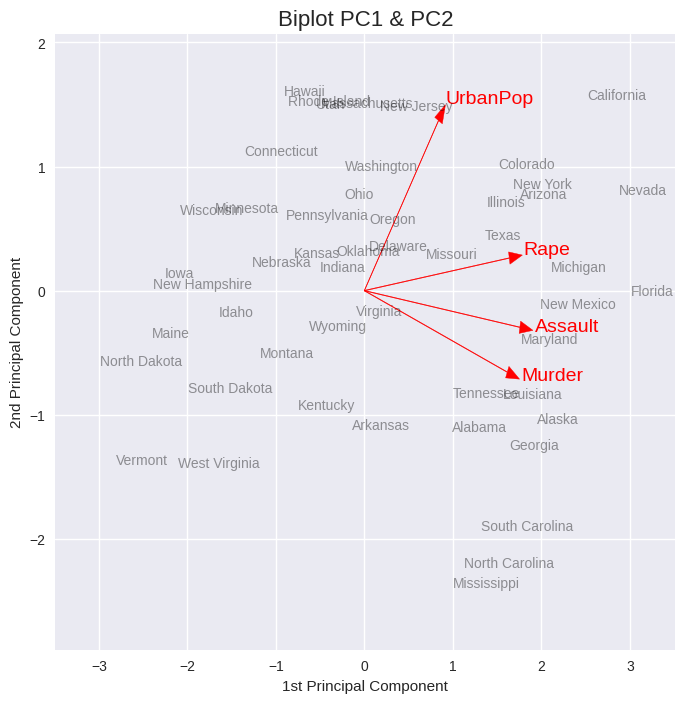
# 0,1 denote PC1 and PC2; change values for other PCs
xvector = pca.components_[0] # see 'prcomp(my_data)$rotation' in R
yvector = -pca.components_[1]

xs = pca.transform(usarrests_scaled)[:,0] # see 'prcomp(my_data)$x' in R
ys = -pca.transform(usarrests_scaled)[:,1]

## visualize projections

plt.figure(figsize=(8, 8))

for i in range(len(xvector)):
# arrows project features (ie columns from csv) as vectors onto PC axes
    plt.arrow(0, 0, xvector[i]*max(xs), yvector[i]*max(ys),
              color='r', width=0.005, head_width=0.1)
    plt.text(xvector[i]*max(xs)*1.1, yvector[i]*max(ys)*1.1,
             usarrests.columns[i], color='r', size=14)

for i in range(len(xs)):
# circles project documents (ie rows from csv) as points onto PC axes
    # plt.plot(xs[i], ys[i], 'bo')
    plt.text(xs[i], ys[i], usarrests.index[i], color='black', alpha=0.4)
    
plt.title('Biplot PC1 & PC2', size=16)    
plt.xlabel('1st Principal Component')
plt.ylabel('2nd Principal Component')

m = 0.5
plt.xlim(min(xs) - m, max(xs) + m)
plt.ylim(min(ys) - m, max(ys) + m);

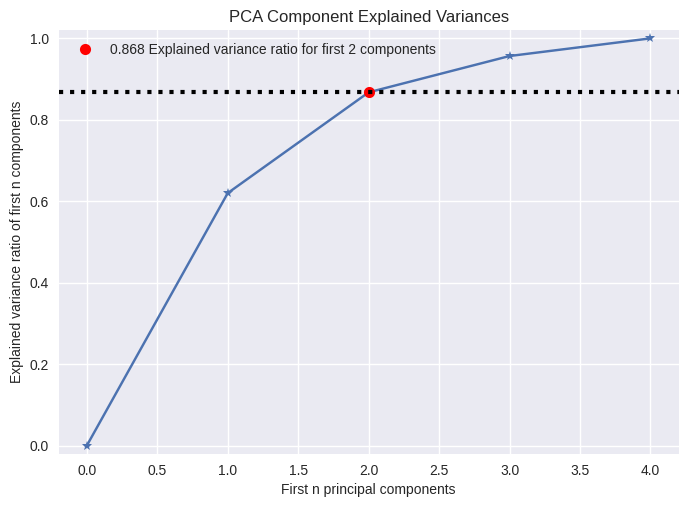
pca.explained_variance_, pca.explained_variance_ratio_

(array([2.53085875, 1.00996444, 0.36383998, 0.17696948]),
 array([0.62006039, 0.24744129, 0.0891408 , 0.04335752]))

from scikitplot.decomposition import plot_pca_component_variance

plot_pca_component_variance(pca, target_explained_variance=0.8);

12.5.2 Matrix Completion

12.5.3 Clustering

K-Means Clustering

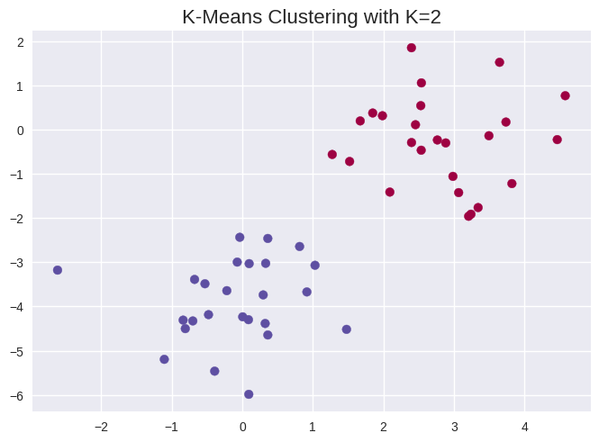
np.random.seed(42)

x = np.random.normal(size=50*2).reshape(50, 2)
x[0:25, 0] += 3
x[25:50, 1] -= 4

from sklearn.cluster import KMeans

kmeans = KMeans(n_clusters=2, random_state=42, n_init=20)
kmeans.fit(x)

KMeans(n_clusters=2, n_init=20, random_state=42)

In a Jupyter environment, please rerun this cell to show the HTML representation or trust the notebook.
On GitHub, the HTML representation is unable to render, please try loading this page with nbviewer.org.

kmeans.labels_

array([0, 0, 0, 0, 0, 0, 0, 0, 0, 0, 0, 0, 0, 0, 0, 0, 0, 0, 0, 0, 0, 0,
       0, 0, 0, 1, 1, 1, 1, 1, 1, 1, 1, 1, 1, 1, 1, 1, 1, 1, 1, 1, 1, 1,
       1, 1, 1, 1, 1, 1], dtype=int32)

plt.scatter(x[:, 0], x[:, 1], c=kmeans.labels_, cmap='Spectral')
plt.title('K-Means Clustering with K=2', size=16);

kmeans2 = KMeans(n_clusters=3, random_state=42, n_init=20)
kmeans2.fit(x)

KMeans(n_clusters=3, n_init=20, random_state=42)

In a Jupyter environment, please rerun this cell to show the HTML representation or trust the notebook.
On GitHub, the HTML representation is unable to render, please try loading this page with nbviewer.org.

kmeans2.cluster_centers_

array([[-0.09155989, -3.87287837],
       [ 3.27858059, -1.37217166],
       [ 2.60450418,  0.24696837]])

kmeans2.labels_

array([2, 2, 2, 2, 2, 2, 1, 2, 2, 1, 1, 1, 2, 2, 2, 2, 1, 1, 1, 2, 2, 2,
       2, 2, 1, 0, 0, 0, 0, 0, 0, 0, 0, 0, 0, 0, 0, 0, 0, 0, 0, 0, 0, 0,
       0, 0, 0, 0, 0, 0], dtype=int32)

kmeans3 = KMeans(n_clusters=3, random_state=42, n_init=1)
kmeans3.fit(x)
kmeans4 = KMeans(n_clusters=3, random_state=42, n_init=20)
kmeans4.fit(x)

print('inertia with n_init=1:', kmeans3.inertia_)
print('inertia with n_init=20:', kmeans4.inertia_)

inertia with n_init=1: 63.70668423951797
inertia with n_init=20: 62.73737809735573

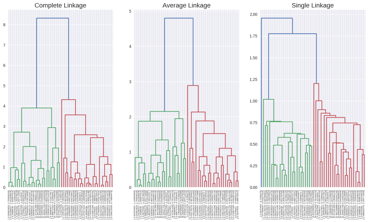
Hierarchical Clustering

from scipy.cluster.hierarchy import linkage, dendrogram

hc_complete = linkage(x, method='complete')
hc_average = linkage(x, method='average')
hc_single = linkage(x, method='single')

f, axes = plt.subplots(1, 3, sharex=False, sharey=False)

f.set_figheight(8)
f.set_figwidth(16)

dendrogram(hc_complete,
           labels=x,
           leaf_rotation=90,
           leaf_font_size=6,
           ax=axes[0])

dendrogram(hc_average,
           labels=x,
           leaf_rotation=90,
           leaf_font_size=6,
           ax=axes[1])

dendrogram(hc_single,
           labels=x,
           leaf_rotation=90,
           leaf_font_size=6,
           ax=axes[2])

axes[0].set_title('Complete Linkage', size=16)
axes[1].set_title('Average Linkage', size=16)
axes[2].set_title('Single Linkage', size=16);

/opt/hostedtoolcache/Python/3.8.18/x64/lib/python3.8/site-packages/matplotlib/text.py:1279: FutureWarning: elementwise comparison failed; returning scalar instead, but in the future will perform elementwise comparison
  if s != self._text:

from scipy.cluster.hierarchy import fcluster, cut_tree

cut_tree(hc_complete, 2).ravel()

array([0, 0, 0, 0, 0, 0, 0, 0, 0, 0, 0, 0, 0, 0, 0, 0, 0, 0, 0, 0, 0, 0,
       0, 0, 0, 1, 1, 1, 1, 1, 1, 1, 1, 1, 1, 1, 1, 1, 1, 1, 1, 1, 1, 1,
       1, 1, 1, 1, 1, 1])

cut_tree(hc_average, 2).ravel()

array([0, 0, 0, 0, 0, 0, 0, 0, 0, 0, 0, 0, 0, 0, 0, 0, 0, 0, 0, 0, 0, 0,
       0, 0, 0, 1, 1, 1, 1, 1, 1, 1, 1, 1, 1, 1, 1, 1, 1, 1, 1, 1, 1, 1,
       1, 1, 1, 1, 1, 1])

cut_tree(hc_single, 2).ravel()

array([0, 0, 0, 0, 0, 0, 0, 0, 0, 0, 0, 0, 0, 0, 0, 0, 0, 0, 0, 0, 0, 0,
       0, 0, 0, 0, 0, 0, 0, 0, 0, 0, 0, 0, 0, 0, 0, 1, 0, 0, 0, 0, 0, 0,
       0, 0, 0, 0, 0, 0])

cut_tree(hc_single, 4).ravel()

array([0, 1, 0, 0, 0, 0, 0, 0, 0, 0, 0, 0, 0, 0, 0, 0, 0, 0, 0, 0, 0, 0,
       0, 0, 0, 2, 2, 2, 2, 2, 2, 2, 2, 2, 2, 2, 2, 3, 2, 2, 2, 2, 2, 2,
       2, 2, 2, 2, 2, 2])

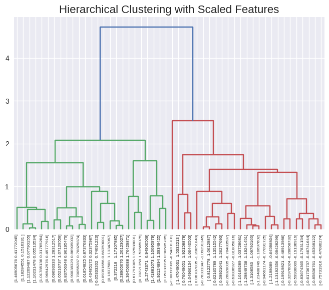
from sklearn.preprocessing import StandardScaler

scaler = StandardScaler()
x_scaled = scaler.fit_transform(x)

dendrogram(linkage(x_scaled, method='complete'),
           labels=x_scaled,
           leaf_rotation=90,
           leaf_font_size=6)

plt.title('Hierarchical Clustering with Scaled Features', size=16);

/opt/hostedtoolcache/Python/3.8.18/x64/lib/python3.8/site-packages/matplotlib/text.py:1279: FutureWarning: elementwise comparison failed; returning scalar instead, but in the future will perform elementwise comparison
  if s != self._text:

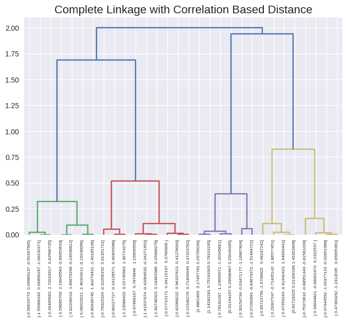
x = np.random.normal(size=30*3).reshape(30, 3)

# scipy linkage takes care of the distance function pdist
dendrogram(linkage(x, method='complete', metric='correlation'),
           labels=x,
           leaf_rotation=90,
           leaf_font_size=6)

plt.title('Complete Linkage with Correlation Based Distance', size=16);

12.5.4: NCI60 Data Example

nci60 = pd.read_csv('../datasets/NCI60.csv', index_col=0)
nci_labs = nci60.labs
nci_data = nci60.drop('labs', axis=1)

nci_data.head()

	data.1	data.2	data.3	data.4	data.5	data.6	...	data.6825	data.6826	data.6827	data.6828	data.6829	data.6830
V1	0.3000	1.1800	0.5500	1.1400	-0.2650	-0.0700	...	0.6300	-0.0300	0.0000	0.2800	-0.3400	-1.9300
V2	0.6800	1.2900	0.1700	0.3800	0.4650	0.5800	...	0.1099	-0.8600	-1.2500	-0.7700	-0.3900	-2.0000
V3	0.9400	-0.0400	-0.1700	-0.0400	-0.6050	0.0000	...	-0.2700	-0.1500	0.0000	-0.1200	-0.4100	0.0000
V4	0.2800	-0.3100	0.6800	-0.8100	0.6250	-0.0000	...	-0.3500	-0.3000	-1.1500	1.0900	-0.2600	-1.1000
V5	0.4850	-0.4650	0.3950	0.9050	0.2000	-0.0050	...	0.6350	0.6050	0.0000	0.7450	0.4250	0.1450

5 rows × 6830 columns

nci_labs.head()

V1       CNS
V2       CNS
V3       CNS
V4     RENAL
V5    BREAST
Name: labs, dtype: object

nci_labs.value_counts()

labs
RENAL          9
NSCLC          9
MELANOMA       8
BREAST         7
COLON          7
              ..
UNKNOWN        1
K562B-repro    1
K562A-repro    1
MCF7A-repro    1
MCF7D-repro    1
Name: count, Length: 14, dtype: int64

PCA on the NCI60 Data

from sklearn.decomposition import PCA
from sklearn.preprocessing import StandardScaler

scaler = StandardScaler()
nci_scaled = scaler.fit_transform(nci_data)

pca = PCA()
pca.fit(nci_scaled)

PCA()

In a Jupyter environment, please rerun this cell to show the HTML representation or trust the notebook.
On GitHub, the HTML representation is unable to render, please try loading this page with nbviewer.org.

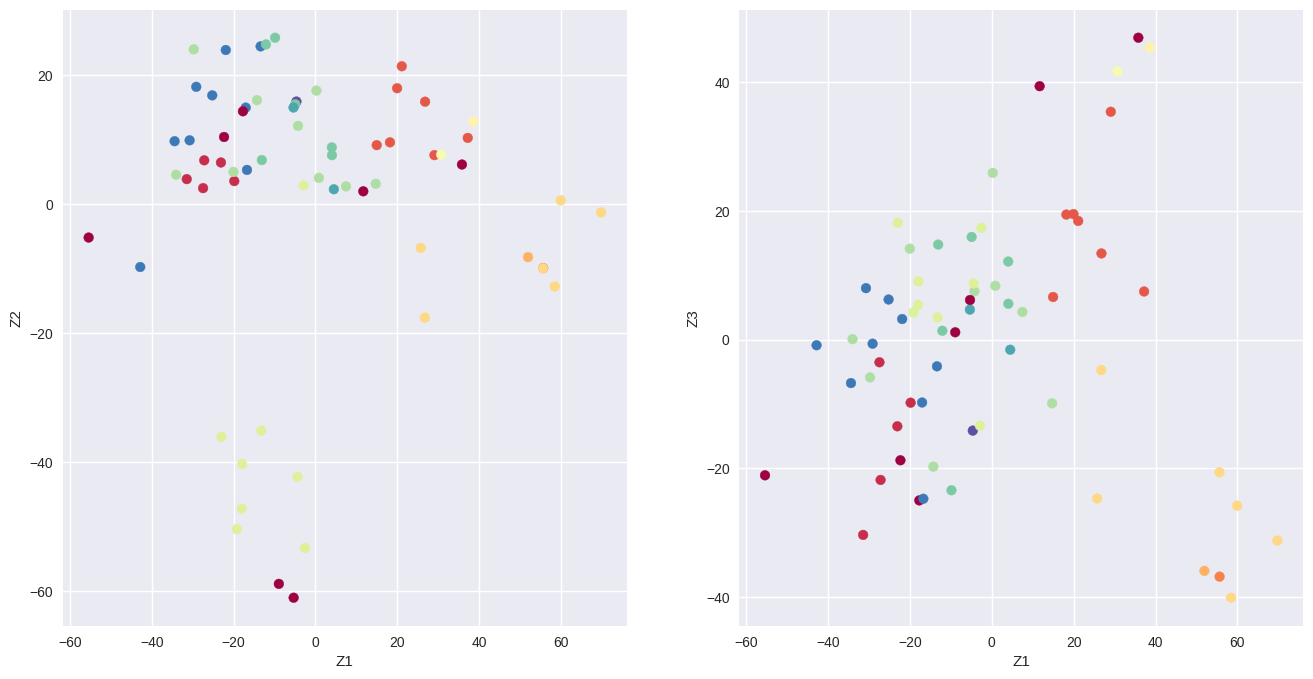
x = pca.transform(nci_scaled)

from sklearn.preprocessing import LabelEncoder

le = LabelEncoder()
color_index = le.fit_transform(nci_labs)

f, axes = plt.subplots(1, 2, sharex=False, sharey=False)

f.set_figheight(8)
f.set_figwidth(16)

axes[0].scatter(x[:, 0], -x[:, 1], c=color_index, cmap='Spectral')
axes[0].set_xlabel('Z1')
axes[0].set_ylabel('Z2')

axes[1].scatter(x[:, 0], x[:, 2], c=color_index, cmap='Spectral')
axes[1].set_xlabel('Z1')
axes[1].set_ylabel('Z3');

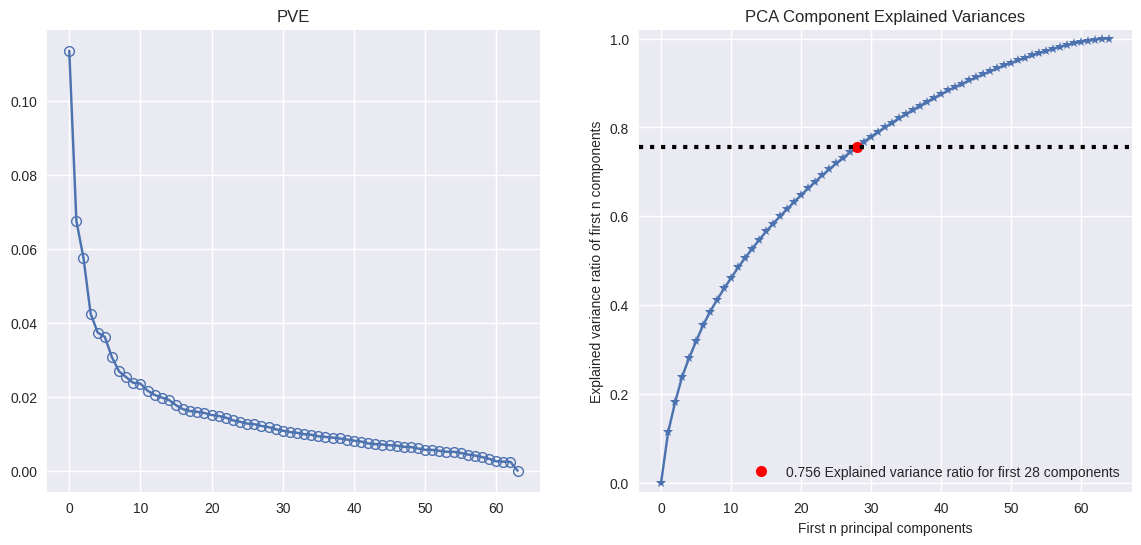
pca.explained_variance_ratio_[:5]

array([0.11358942, 0.06756203, 0.05751842, 0.04247554, 0.03734972])

pca.explained_variance_ratio_.cumsum()[:5]

array([0.11358942, 0.18115144, 0.23866987, 0.28114541, 0.31849513])

from scikitplot.decomposition import plot_pca_component_variance

f, axes = plt.subplots(1, 2, sharex=False, sharey=False)

f.set_figheight(6)
f.set_figwidth(14)

axes[0].plot(pca.explained_variance_ratio_, marker='o', markeredgewidth=1, markerfacecolor='None')
axes[0].set_title('PVE')
plot_pca_component_variance(pca, ax=axes[1]);

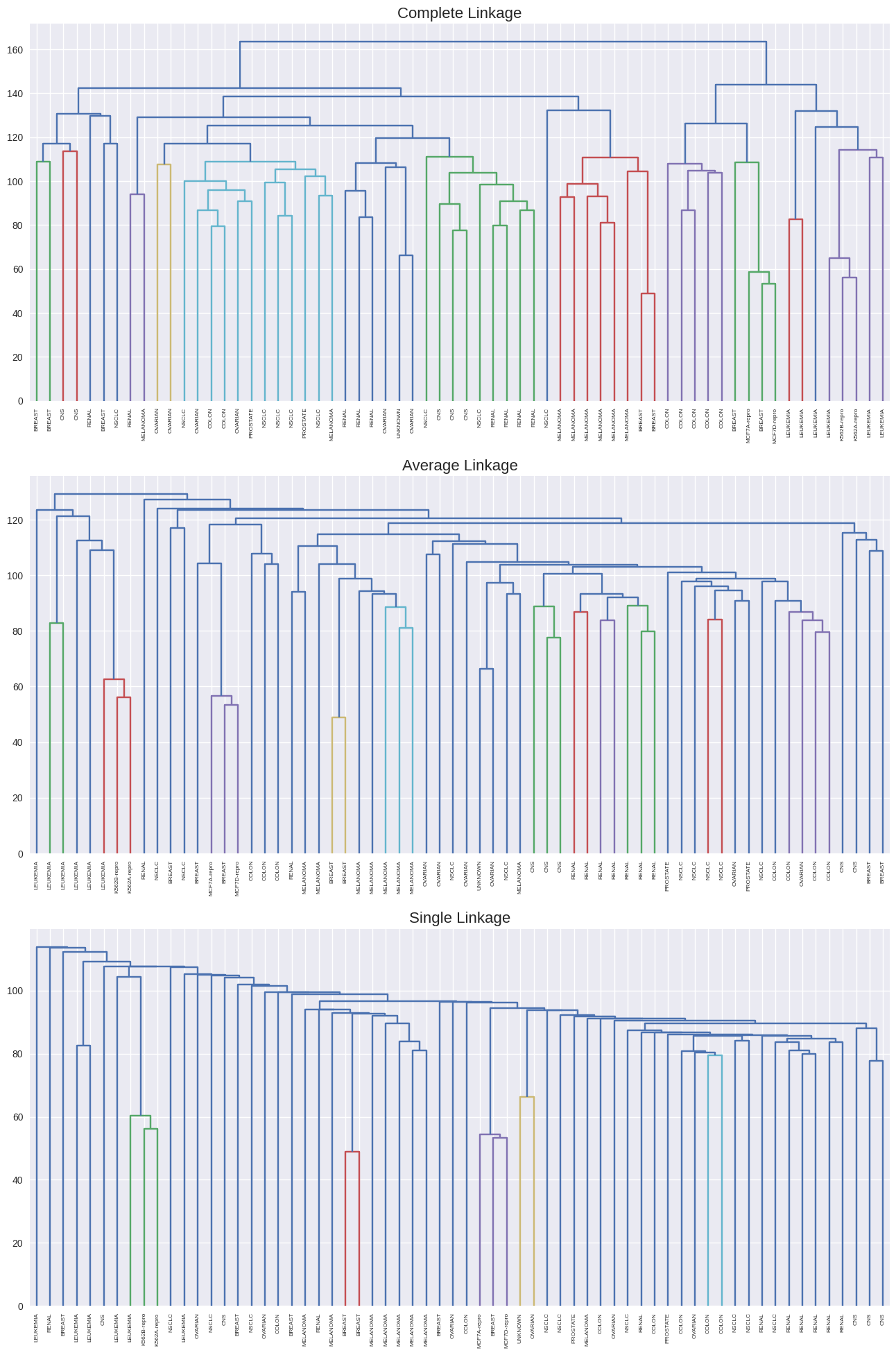
Clustering the Observations of the NCI60 Data

from scipy.cluster.hierarchy import dendrogram, linkage, cut_tree

f, axes = plt.subplots(3, 1, sharex=False, sharey=False)

f.set_figheight(24)
f.set_figwidth(16)

dendrogram(linkage(nci_scaled, method='complete'),
           labels=nci_labs,
           leaf_rotation=90,
           leaf_font_size=6,
           ax=axes[0])

dendrogram(linkage(nci_scaled, method='average'),
           labels=nci_labs,
           leaf_rotation=90,
           leaf_font_size=6,
           ax=axes[1])

dendrogram(linkage(nci_scaled, method='single'),
           labels=nci_labs,
           leaf_rotation=90,
           leaf_font_size=6,
           ax=axes[2])

axes[0].set_title('Complete Linkage', size=16)
axes[1].set_title('Average Linkage', size=16)
axes[2].set_title('Single Linkage', size=16);

hc_clusters = cut_tree(linkage(nci_scaled, method='complete'), 4).ravel()
pd.crosstab(hc_clusters, nci_labs)

labs	BREAST	CNS	COLON	K562A-repro	K562B-repro	LEUKEMIA	...	MELANOMA	NSCLC	OVARIAN	PROSTATE	RENAL	UNKNOWN
row_0
0	2	3	2	0	0	0	...	8	8	6	2	8	1
1	3	2	0	0	0	0	...	0	1	0	0	1	0
2	0	0	0	1	1	6	...	0	0	0	0	0	0
3	2	0	5	0	0	0	...	0	0	0	0	0	0

4 rows × 14 columns

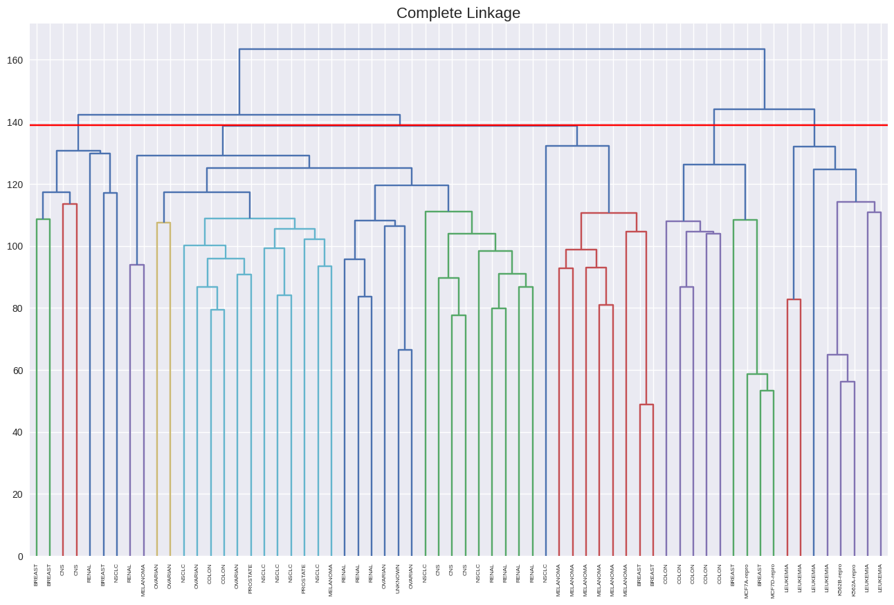
plt.figure(figsize=(16, 10))

dendrogram(linkage(nci_scaled, method='complete'),
           labels=nci_labs,
           leaf_rotation=90,
           leaf_font_size=6)

plt.axhline(y=139, c='r')
plt.title('Complete Linkage', size=16);

from sklearn.cluster import KMeans

km = KMeans(n_clusters=4, n_init=20, random_state=42)
km.fit(nci_scaled)

pd.crosstab(km.labels_, hc_clusters)

col_0	0	1	2	3
row_0
0	9	0	0	0
1	2	0	0	9
2	0	0	8	0
3	29	7	0	0

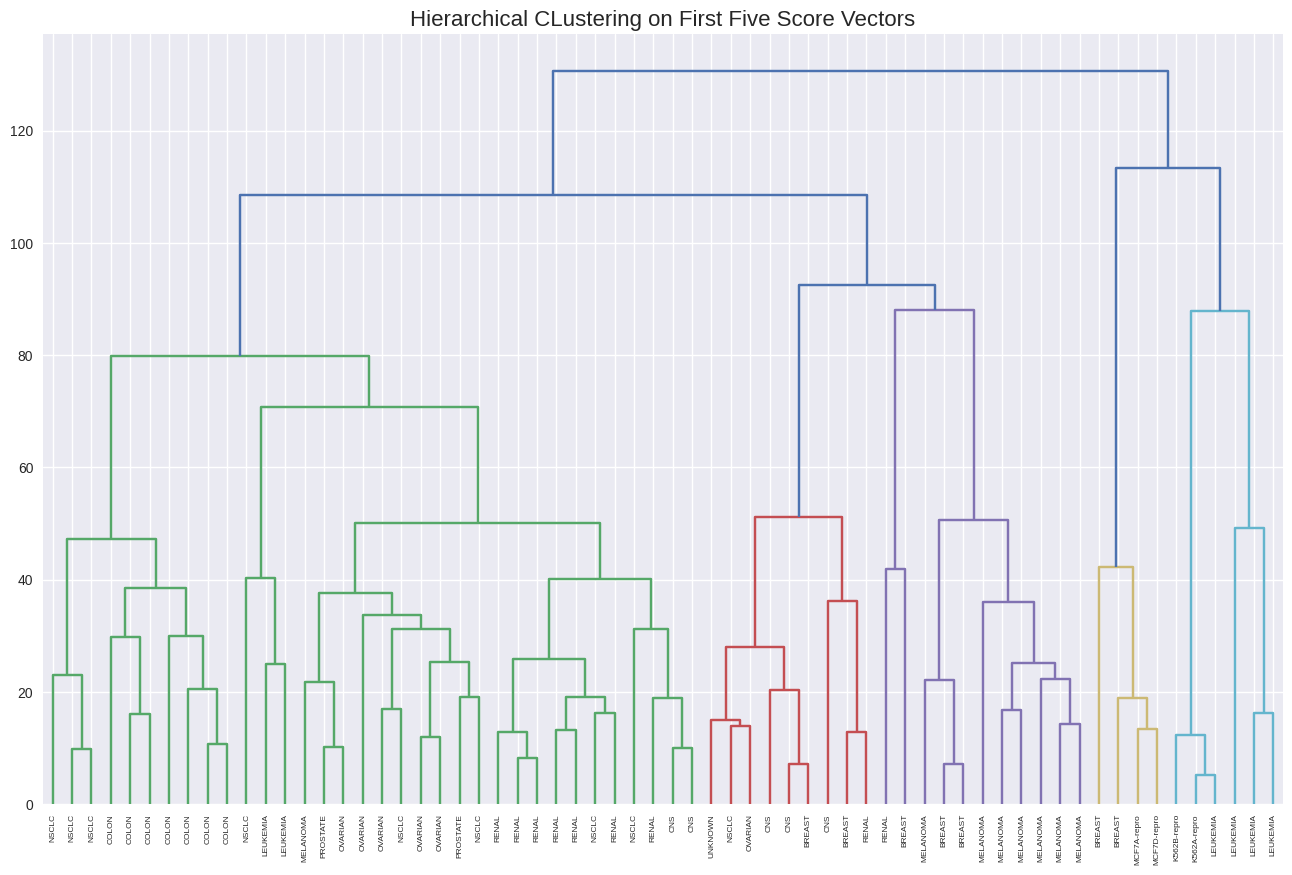
hc2 = linkage(x[:, 0:5], method='complete')

plt.figure(figsize=(16, 10))

dendrogram(hc2,
           labels=nci_labs,
           leaf_rotation=90,
           leaf_font_size=6)

plt.title('Hierarchical CLustering on First Five Score Vectors', size=16);

pd.crosstab(cut_tree(hc2, 4).ravel(), nci_labs)

labs	BREAST	CNS	COLON	K562A-repro	K562B-repro	LEUKEMIA	...	MELANOMA	NSCLC	OVARIAN	PROSTATE	RENAL	UNKNOWN
row_0
0	0	2	7	0	0	2	...	1	8	5	2	7	0
1	5	3	0	0	0	0	...	7	1	1	0	2	1
2	0	0	0	1	1	4	...	0	0	0	0	0	0
3	2	0	0	0	0	0	...	0	0	0	0	0	0

4 rows × 14 columns