Chapter 6 – Decision Trees

This notebook contains all the sample code and solutions to the exercises in chapter 6.

Setup

First, let’s import a few common modules, ensure MatplotLib plots figures inline and prepare a function to save the figures. We also check that Python 3.5 or later is installed (although Python 2.x may work, it is deprecated so we strongly recommend you use Python 3 instead), as well as Scikit-Learn ≥0.20.

# Python ≥3.5 is required
import sys
assert sys.version_info >= (3, 5)

# Scikit-Learn ≥0.20 is required
import sklearn
assert sklearn.__version__ >= "0.20"

# Common imports
import numpy as np
import os

# to make this notebook's output stable across runs
np.random.seed(42)

# To plot pretty figures
%matplotlib inline
import matplotlib as mpl
import matplotlib.pyplot as plt
mpl.rc('axes', labelsize=14)
mpl.rc('xtick', labelsize=12)
mpl.rc('ytick', labelsize=12)

# Where to save the figures
PROJECT_ROOT_DIR = "."
CHAPTER_ID = "decision_trees"
IMAGES_PATH = os.path.join(PROJECT_ROOT_DIR, "images", CHAPTER_ID)
os.makedirs(IMAGES_PATH, exist_ok=True)

def save_fig(fig_id, tight_layout=True, fig_extension="png", resolution=300):
    path = os.path.join(IMAGES_PATH, fig_id + "." + fig_extension)
    print("Saving figure", fig_id)
    if tight_layout:
        plt.tight_layout()
    plt.savefig(path, format=fig_extension, dpi=resolution)

Training and Visualizing a Decision Tree

from sklearn.datasets import load_iris
from sklearn.tree import DecisionTreeClassifier

iris = load_iris()
X = iris.data[:, 2:] # petal length and width
y = iris.target

tree_clf = DecisionTreeClassifier(max_depth=2, random_state=42)
tree_clf.fit(X, y)

DecisionTreeClassifier(max_depth=2, random_state=42)

This code example generates Figure 6–1. Iris Decision Tree:

from graphviz import Source
from sklearn.tree import export_graphviz

export_graphviz(
        tree_clf,
        out_file=os.path.join(IMAGES_PATH, "iris_tree.dot"),
        feature_names=iris.feature_names[2:],
        class_names=iris.target_names,
        rounded=True,
        filled=True
    )

Source.from_file(os.path.join(IMAGES_PATH, "iris_tree.dot"))

Making Predictions

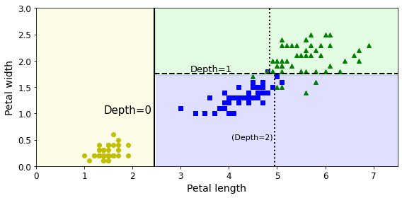
Code to generate Figure 6–2. Decision Tree decision boundaries

from matplotlib.colors import ListedColormap

def plot_decision_boundary(clf, X, y, axes=[0, 7.5, 0, 3], iris=True, legend=False, plot_training=True):
    x1s = np.linspace(axes[0], axes[1], 100)
    x2s = np.linspace(axes[2], axes[3], 100)
    x1, x2 = np.meshgrid(x1s, x2s)
    X_new = np.c_[x1.ravel(), x2.ravel()]
    y_pred = clf.predict(X_new).reshape(x1.shape)
    custom_cmap = ListedColormap(['#fafab0','#9898ff','#a0faa0'])
    plt.contourf(x1, x2, y_pred, alpha=0.3, cmap=custom_cmap)
    if not iris:
        custom_cmap2 = ListedColormap(['#7d7d58','#4c4c7f','#507d50'])
        plt.contour(x1, x2, y_pred, cmap=custom_cmap2, alpha=0.8)
    if plot_training:
        plt.plot(X[:, 0][y==0], X[:, 1][y==0], "yo", label="Iris setosa")
        plt.plot(X[:, 0][y==1], X[:, 1][y==1], "bs", label="Iris versicolor")
        plt.plot(X[:, 0][y==2], X[:, 1][y==2], "g^", label="Iris virginica")
        plt.axis(axes)
    if iris:
        plt.xlabel("Petal length", fontsize=14)
        plt.ylabel("Petal width", fontsize=14)
    else:
        plt.xlabel(r"$x_1$", fontsize=18)
        plt.ylabel(r"$x_2$", fontsize=18, rotation=0)
    if legend:
        plt.legend(loc="lower right", fontsize=14)

plt.figure(figsize=(8, 4))
plot_decision_boundary(tree_clf, X, y)
plt.plot([2.45, 2.45], [0, 3], "k-", linewidth=2)
plt.plot([2.45, 7.5], [1.75, 1.75], "k--", linewidth=2)
plt.plot([4.95, 4.95], [0, 1.75], "k:", linewidth=2)
plt.plot([4.85, 4.85], [1.75, 3], "k:", linewidth=2)
plt.text(1.40, 1.0, "Depth=0", fontsize=15)
plt.text(3.2, 1.80, "Depth=1", fontsize=13)
plt.text(4.05, 0.5, "(Depth=2)", fontsize=11)

save_fig("decision_tree_decision_boundaries_plot")
plt.show()

Saving figure decision_tree_decision_boundaries_plot

Estimating Class Probabilities

tree_clf.predict_proba([[5, 1.5]])

array([[0.        , 0.90740741, 0.09259259]])

tree_clf.predict([[5, 1.5]])

array([1])

Regularization Hyperparameters

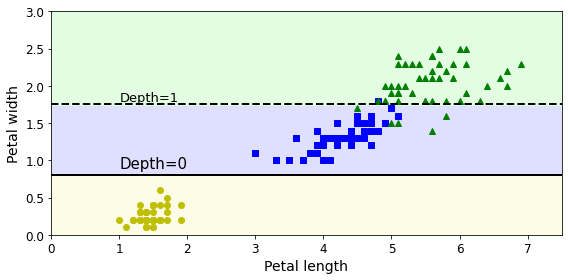
We’ve seen that small changes in the dataset (such as a rotation) may produce a very different Decision Tree. Now let’s show that training the same model on the same data may produce a very different model every time, since the CART training algorithm used by Scikit-Learn is stochastic. To show this, we will set random_state to a different value than earlier:

tree_clf_tweaked = DecisionTreeClassifier(max_depth=2, random_state=40)
tree_clf_tweaked.fit(X, y)

DecisionTreeClassifier(max_depth=2, random_state=40)

Code to generate Figure 6–8. Sensitivity to training set details:

plt.figure(figsize=(8, 4))
plot_decision_boundary(tree_clf_tweaked, X, y, legend=False)
plt.plot([0, 7.5], [0.8, 0.8], "k-", linewidth=2)
plt.plot([0, 7.5], [1.75, 1.75], "k--", linewidth=2)
plt.text(1.0, 0.9, "Depth=0", fontsize=15)
plt.text(1.0, 1.80, "Depth=1", fontsize=13)

save_fig("decision_tree_instability_plot")
plt.show()

Saving figure decision_tree_instability_plot

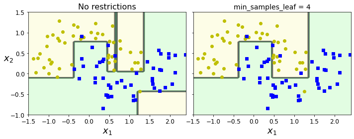
Code to generate Figure 6–3. Regularization using min_samples_leaf:

from sklearn.datasets import make_moons
Xm, ym = make_moons(n_samples=100, noise=0.25, random_state=53)

deep_tree_clf1 = DecisionTreeClassifier(random_state=42)
deep_tree_clf2 = DecisionTreeClassifier(min_samples_leaf=4, random_state=42)
deep_tree_clf1.fit(Xm, ym)
deep_tree_clf2.fit(Xm, ym)

fig, axes = plt.subplots(ncols=2, figsize=(10, 4), sharey=True)
plt.sca(axes[0])
plot_decision_boundary(deep_tree_clf1, Xm, ym, axes=[-1.5, 2.4, -1, 1.5], iris=False)
plt.title("No restrictions", fontsize=16)
plt.sca(axes[1])
plot_decision_boundary(deep_tree_clf2, Xm, ym, axes=[-1.5, 2.4, -1, 1.5], iris=False)
plt.title("min_samples_leaf = {}".format(deep_tree_clf2.min_samples_leaf), fontsize=14)
plt.ylabel("")

save_fig("min_samples_leaf_plot")
plt.show()

Saving figure min_samples_leaf_plot

Rotating the dataset also leads to completely different decision boundaries:

angle = np.pi / 180 * 20
rotation_matrix = np.array([[np.cos(angle), -np.sin(angle)], [np.sin(angle), np.cos(angle)]])
Xr = X.dot(rotation_matrix)

tree_clf_r = DecisionTreeClassifier(random_state=42)
tree_clf_r.fit(Xr, y)

plt.figure(figsize=(8, 3))
plot_decision_boundary(tree_clf_r, Xr, y, axes=[0.5, 7.5, -1.0, 1], iris=False)

plt.show()

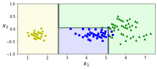
Code to generate Figure 6–7. Sensitivity to training set rotation

np.random.seed(6)
Xs = np.random.rand(100, 2) - 0.5
ys = (Xs[:, 0] > 0).astype(np.float32) * 2

angle = np.pi / 4
rotation_matrix = np.array([[np.cos(angle), -np.sin(angle)], [np.sin(angle), np.cos(angle)]])
Xsr = Xs.dot(rotation_matrix)

tree_clf_s = DecisionTreeClassifier(random_state=42)
tree_clf_s.fit(Xs, ys)
tree_clf_sr = DecisionTreeClassifier(random_state=42)
tree_clf_sr.fit(Xsr, ys)

fig, axes = plt.subplots(ncols=2, figsize=(10, 4), sharey=True)
plt.sca(axes[0])
plot_decision_boundary(tree_clf_s, Xs, ys, axes=[-0.7, 0.7, -0.7, 0.7], iris=False)
plt.sca(axes[1])
plot_decision_boundary(tree_clf_sr, Xsr, ys, axes=[-0.7, 0.7, -0.7, 0.7], iris=False)
plt.ylabel("")

save_fig("sensitivity_to_rotation_plot")
plt.show()

Saving figure sensitivity_to_rotation_plot

Regression

Let’s prepare a simple linear dataset:

# Quadratic training set + noise
np.random.seed(42)
m = 200
X = np.random.rand(m, 1)
y = 4 * (X - 0.5) ** 2
y = y + np.random.randn(m, 1) / 10

Code example:

from sklearn.tree import DecisionTreeRegressor

tree_reg = DecisionTreeRegressor(max_depth=2, random_state=42)
tree_reg.fit(X, y)

DecisionTreeRegressor(max_depth=2, random_state=42)

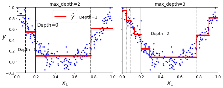
Code to generate Figure 6–5. Predictions of two Decision Tree regression models:

from sklearn.tree import DecisionTreeRegressor

tree_reg1 = DecisionTreeRegressor(random_state=42, max_depth=2)
tree_reg2 = DecisionTreeRegressor(random_state=42, max_depth=3)
tree_reg1.fit(X, y)
tree_reg2.fit(X, y)

def plot_regression_predictions(tree_reg, X, y, axes=[0, 1, -0.2, 1], ylabel="$y$"):
    x1 = np.linspace(axes[0], axes[1], 500).reshape(-1, 1)
    y_pred = tree_reg.predict(x1)
    plt.axis(axes)
    plt.xlabel("$x_1$", fontsize=18)
    if ylabel:
        plt.ylabel(ylabel, fontsize=18, rotation=0)
    plt.plot(X, y, "b.")
    plt.plot(x1, y_pred, "r.-", linewidth=2, label=r"$\hat{y}$")

fig, axes = plt.subplots(ncols=2, figsize=(10, 4), sharey=True)
plt.sca(axes[0])
plot_regression_predictions(tree_reg1, X, y)
for split, style in ((0.1973, "k-"), (0.0917, "k--"), (0.7718, "k--")):
    plt.plot([split, split], [-0.2, 1], style, linewidth=2)
plt.text(0.21, 0.65, "Depth=0", fontsize=15)
plt.text(0.01, 0.2, "Depth=1", fontsize=13)
plt.text(0.65, 0.8, "Depth=1", fontsize=13)
plt.legend(loc="upper center", fontsize=18)
plt.title("max_depth=2", fontsize=14)

plt.sca(axes[1])
plot_regression_predictions(tree_reg2, X, y, ylabel=None)
for split, style in ((0.1973, "k-"), (0.0917, "k--"), (0.7718, "k--")):
    plt.plot([split, split], [-0.2, 1], style, linewidth=2)
for split in (0.0458, 0.1298, 0.2873, 0.9040):
    plt.plot([split, split], [-0.2, 1], "k:", linewidth=1)
plt.text(0.3, 0.5, "Depth=2", fontsize=13)
plt.title("max_depth=3", fontsize=14)

save_fig("tree_regression_plot")
plt.show()

Saving figure tree_regression_plot

Code to generate Figure 6-4. A Decision Tree for regression:

export_graphviz(
        tree_reg1,
        out_file=os.path.join(IMAGES_PATH, "regression_tree.dot"),
        feature_names=["x1"],
        rounded=True,
        filled=True
    )

Source.from_file(os.path.join(IMAGES_PATH, "regression_tree.dot"))

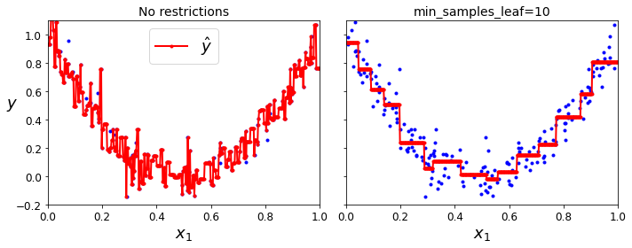
Code to generate Figure 6–6. Regularizing a Decision Tree regressor:

tree_reg1 = DecisionTreeRegressor(random_state=42)
tree_reg2 = DecisionTreeRegressor(random_state=42, min_samples_leaf=10)
tree_reg1.fit(X, y)
tree_reg2.fit(X, y)

x1 = np.linspace(0, 1, 500).reshape(-1, 1)
y_pred1 = tree_reg1.predict(x1)
y_pred2 = tree_reg2.predict(x1)

fig, axes = plt.subplots(ncols=2, figsize=(10, 4), sharey=True)

plt.sca(axes[0])
plt.plot(X, y, "b.")
plt.plot(x1, y_pred1, "r.-", linewidth=2, label=r"$\hat{y}$")
plt.axis([0, 1, -0.2, 1.1])
plt.xlabel("$x_1$", fontsize=18)
plt.ylabel("$y$", fontsize=18, rotation=0)
plt.legend(loc="upper center", fontsize=18)
plt.title("No restrictions", fontsize=14)

plt.sca(axes[1])
plt.plot(X, y, "b.")
plt.plot(x1, y_pred2, "r.-", linewidth=2, label=r"$\hat{y}$")
plt.axis([0, 1, -0.2, 1.1])
plt.xlabel("$x_1$", fontsize=18)
plt.title("min_samples_leaf={}".format(tree_reg2.min_samples_leaf), fontsize=14)

save_fig("tree_regression_regularization_plot")
plt.show()

Saving figure tree_regression_regularization_plot

Exercise solutions

1. to 6.

See appendix A.

7.

Exercise: train and fine-tune a Decision Tree for the moons dataset.

a. Generate a moons dataset using make_moons(n_samples=10000, noise=0.4).

Adding random_state=42 to make this notebook’s output constant:

from sklearn.datasets import make_moons

X, y = make_moons(n_samples=10000, noise=0.4, random_state=42)

b. Split it into a training set and a test set using train_test_split().

from sklearn.model_selection import train_test_split

X_train, X_test, y_train, y_test = train_test_split(X, y, test_size=0.2, random_state=42)

c. Use grid search with cross-validation (with the help of the GridSearchCV class) to find good hyperparameter values for a DecisionTreeClassifier. Hint: try various values for max_leaf_nodes.

from sklearn.model_selection import GridSearchCV

params = {'max_leaf_nodes': list(range(2, 100)), 'min_samples_split': [2, 3, 4]}
grid_search_cv = GridSearchCV(DecisionTreeClassifier(random_state=42), params, verbose=1, cv=3)

grid_search_cv.fit(X_train, y_train)

Fitting 3 folds for each of 294 candidates, totalling 882 fits

[Parallel(n_jobs=1)]: Using backend SequentialBackend with 1 concurrent workers.
[Parallel(n_jobs=1)]: Done 882 out of 882 | elapsed:    5.7s finished

GridSearchCV(cv=3, estimator=DecisionTreeClassifier(random_state=42),
             param_grid={'max_leaf_nodes': [2, 3, 4, 5, 6, 7, 8, 9, 10, 11, 12,
                                            13, 14, 15, 16, 17, 18, 19, 20, 21,
                                            22, 23, 24, 25, 26, 27, 28, 29, 30,
                                            31, ...],
                         'min_samples_split': [2, 3, 4]},
             verbose=1)

grid_search_cv.best_estimator_

DecisionTreeClassifier(max_leaf_nodes=17, random_state=42)

d. Train it on the full training set using these hyperparameters, and measure your model’s performance on the test set. You should get roughly 85% to 87% accuracy.

By default, GridSearchCV trains the best model found on the whole training set (you can change this by setting refit=False), so we don’t need to do it again. We can simply evaluate the model’s accuracy:

from sklearn.metrics import accuracy_score

y_pred = grid_search_cv.predict(X_test)
accuracy_score(y_test, y_pred)

0.8695

8.

Exercise: Grow a forest.

a. Continuing the previous exercise, generate 1,000 subsets of the training set, each containing 100 instances selected randomly. Hint: you can use Scikit-Learn’s ShuffleSplit class for this.

from sklearn.model_selection import ShuffleSplit

n_trees = 1000
n_instances = 100

mini_sets = []

rs = ShuffleSplit(n_splits=n_trees, test_size=len(X_train) - n_instances, random_state=42)
for mini_train_index, mini_test_index in rs.split(X_train):
    X_mini_train = X_train[mini_train_index]
    y_mini_train = y_train[mini_train_index]
    mini_sets.append((X_mini_train, y_mini_train))

b. Train one Decision Tree on each subset, using the best hyperparameter values found above. Evaluate these 1,000 Decision Trees on the test set. Since they were trained on smaller sets, these Decision Trees will likely perform worse than the first Decision Tree, achieving only about 80% accuracy.

from sklearn.base import clone

forest = [clone(grid_search_cv.best_estimator_) for _ in range(n_trees)]

accuracy_scores = []

for tree, (X_mini_train, y_mini_train) in zip(forest, mini_sets):
    tree.fit(X_mini_train, y_mini_train)
    
    y_pred = tree.predict(X_test)
    accuracy_scores.append(accuracy_score(y_test, y_pred))

np.mean(accuracy_scores)

0.8054499999999999

c. Now comes the magic. For each test set instance, generate the predictions of the 1,000 Decision Trees, and keep only the most frequent prediction (you can use SciPy’s mode() function for this). This gives you majority-vote predictions over the test set.

Y_pred = np.empty([n_trees, len(X_test)], dtype=np.uint8)

for tree_index, tree in enumerate(forest):
    Y_pred[tree_index] = tree.predict(X_test)

from scipy.stats import mode

y_pred_majority_votes, n_votes = mode(Y_pred, axis=0)

d. Evaluate these predictions on the test set: you should obtain a slightly higher accuracy than your first model (about 0.5 to 1.5% higher). Congratulations, you have trained a Random Forest classifier!

accuracy_score(y_test, y_pred_majority_votes.reshape([-1]))

0.872