Chapter 17 – Autoencoders and GANs**#
This notebook contains all the sample code in chapter 17.
Setup#
First, let’s import a few common modules, ensure MatplotLib plots figures inline and prepare a function to save the figures. We also check that Python 3.5 or later is installed (although Python 2.x may work, it is deprecated so we strongly recommend you use Python 3 instead), as well as Scikit-Learn ≥0.20 and TensorFlow ≥2.0.
# Python ≥3.5 is required
import sys
assert sys.version_info >= (3, 5)

# Is this notebook running on Colab or Kaggle?
IS_COLAB = "google.colab" in sys.modules
IS_KAGGLE = "kaggle_secrets" in sys.modules

# Scikit-Learn ≥0.20 is required
import sklearn
assert sklearn.__version__ >= "0.20"

# TensorFlow ≥2.0 is required
import tensorflow as tf
from tensorflow import keras
assert tf.__version__ >= "2.0"

if not tf.config.list_physical_devices('GPU'):
    print("No GPU was detected. LSTMs and CNNs can be very slow without a GPU.")
    if IS_COLAB:
        print("Go to Runtime > Change runtime and select a GPU hardware accelerator.")
    if IS_KAGGLE:
        print("Go to Settings > Accelerator and select GPU.")

# Common imports
import numpy as np
import os

# to make this notebook's output stable across runs
np.random.seed(42)
tf.random.set_seed(42)

# To plot pretty figures
%matplotlib inline
import matplotlib as mpl
import matplotlib.pyplot as plt
mpl.rc('axes', labelsize=14)
mpl.rc('xtick', labelsize=12)
mpl.rc('ytick', labelsize=12)

# Where to save the figures
PROJECT_ROOT_DIR = "."
CHAPTER_ID = "autoencoders"
IMAGES_PATH = os.path.join(PROJECT_ROOT_DIR, "images", CHAPTER_ID)
os.makedirs(IMAGES_PATH, exist_ok=True)

def save_fig(fig_id, tight_layout=True, fig_extension="png", resolution=300):
    path = os.path.join(IMAGES_PATH, fig_id + "." + fig_extension)
    print("Saving figure", fig_id)
    if tight_layout:
        plt.tight_layout()
    plt.savefig(path, format=fig_extension, dpi=resolution)
No GPU was detected. LSTMs and CNNs can be very slow without a GPU.
A couple utility functions to plot grayscale 28x28 image:
def plot_image(image):
    plt.imshow(image, cmap="binary")
    plt.axis("off")
PCA with a linear Autoencoder#
Build 3D dataset:
np.random.seed(4)

def generate_3d_data(m, w1=0.1, w2=0.3, noise=0.1):
    angles = np.random.rand(m) * 3 * np.pi / 2 - 0.5
    data = np.empty((m, 3))
    data[:, 0] = np.cos(angles) + np.sin(angles)/2 + noise * np.random.randn(m) / 2
    data[:, 1] = np.sin(angles) * 0.7 + noise * np.random.randn(m) / 2
    data[:, 2] = data[:, 0] * w1 + data[:, 1] * w2 + noise * np.random.randn(m)
    return data

X_train = generate_3d_data(60)
X_train = X_train - X_train.mean(axis=0, keepdims=0)
Now let’s build the Autoencoder…
np.random.seed(42)
tf.random.set_seed(42)

encoder = keras.models.Sequential([keras.layers.Dense(2, input_shape=[3])])
decoder = keras.models.Sequential([keras.layers.Dense(3, input_shape=[2])])
autoencoder = keras.models.Sequential([encoder, decoder])

autoencoder.compile(loss="mse", optimizer=keras.optimizers.SGD(learning_rate=1.5))
history = autoencoder.fit(X_train, X_train, epochs=20)
Train on 60 samples
Epoch 1/20
60/60 [==============================] - 0s 1ms/sample - loss: 0.2648
Epoch 2/20
60/60 [==============================] - 0s 49us/sample - loss: 0.1317
Epoch 3/20
60/60 [==============================] - 0s 50us/sample - loss: 0.0778
Epoch 4/20
60/60 [==============================] - 0s 46us/sample - loss: 0.0655
Epoch 5/20
60/60 [==============================] - 0s 51us/sample - loss: 0.0748
Epoch 6/20
60/60 [==============================] - 0s 47us/sample - loss: 0.1039
Epoch 7/20
60/60 [==============================] - 0s 50us/sample - loss: 0.1262
Epoch 8/20
60/60 [==============================] - 0s 52us/sample - loss: 0.0536
Epoch 9/20
60/60 [==============================] - 0s 51us/sample - loss: 0.0208
Epoch 10/20
60/60 [==============================] - 0s 52us/sample - loss: 0.0146
Epoch 11/20
60/60 [==============================] - 0s 52us/sample - loss: 0.0097
Epoch 12/20
60/60 [==============================] - 0s 48us/sample - loss: 0.0076
Epoch 13/20
60/60 [==============================] - 0s 43us/sample - loss: 0.0067
Epoch 14/20
60/60 [==============================] - 0s 49us/sample - loss: 0.0070
Epoch 15/20
60/60 [==============================] - 0s 58us/sample - loss: 0.0061
Epoch 16/20
60/60 [==============================] - 0s 53us/sample - loss: 0.0055
Epoch 17/20
60/60 [==============================] - 0s 63us/sample - loss: 0.0056
Epoch 18/20
60/60 [==============================] - 0s 58us/sample - loss: 0.0055
Epoch 19/20
60/60 [==============================] - 0s 64us/sample - loss: 0.0054
Epoch 20/20
60/60 [==============================] - 0s 55us/sample - loss: 0.0055
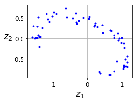
codings = encoder.predict(X_train)
fig = plt.figure(figsize=(4,3))
plt.plot(codings[:,0], codings[:, 1], "b.")
plt.xlabel("$z_1$", fontsize=18)
plt.ylabel("$z_2$", fontsize=18, rotation=0)
plt.grid(True)
save_fig("linear_autoencoder_pca_plot")
plt.show()
Saving figure linear_autoencoder_pca_plot
Stacked Autoencoders#
Let’s use MNIST:
(X_train_full, y_train_full), (X_test, y_test) = keras.datasets.fashion_mnist.load_data()
X_train_full = X_train_full.astype(np.float32) / 255
X_test = X_test.astype(np.float32) / 255
X_train, X_valid = X_train_full[:-5000], X_train_full[-5000:]
y_train, y_valid = y_train_full[:-5000], y_train_full[-5000:]
Train all layers at once#
Let’s build a stacked Autoencoder with 3 hidden layers and 1 output layer (i.e., 2 stacked Autoencoders).
def rounded_accuracy(y_true, y_pred):
    return keras.metrics.binary_accuracy(tf.round(y_true), tf.round(y_pred))
tf.random.set_seed(42)
np.random.seed(42)

stacked_encoder = keras.models.Sequential([
    keras.layers.Flatten(input_shape=[28, 28]),
    keras.layers.Dense(100, activation="selu"),
    keras.layers.Dense(30, activation="selu"),
])
stacked_decoder = keras.models.Sequential([
    keras.layers.Dense(100, activation="selu", input_shape=[30]),
    keras.layers.Dense(28 * 28, activation="sigmoid"),
    keras.layers.Reshape([28, 28])
])
stacked_ae = keras.models.Sequential([stacked_encoder, stacked_decoder])
stacked_ae.compile(loss="binary_crossentropy",
                   optimizer=keras.optimizers.SGD(learning_rate=1.5), metrics=[rounded_accuracy])
history = stacked_ae.fit(X_train, X_train, epochs=20,
                         validation_data=(X_valid, X_valid))
Train on 55000 samples, validate on 5000 samples
Epoch 1/20
55000/55000 [==============================] - 4s 72us/sample - loss: 0.3386 - rounded_accuracy: 0.8866 - val_loss: 0.3118 - val_rounded_accuracy: 0.9128
Epoch 2/20
55000/55000 [==============================] - 4s 64us/sample - loss: 0.3055 - rounded_accuracy: 0.9153 - val_loss: 0.3030 - val_rounded_accuracy: 0.9200
Epoch 3/20
55000/55000 [==============================] - 4s 68us/sample - loss: 0.2986 - rounded_accuracy: 0.9214 - val_loss: 0.2982 - val_rounded_accuracy: 0.9249
Epoch 4/20
55000/55000 [==============================] - 4s 67us/sample - loss: 0.2946 - rounded_accuracy: 0.9251 - val_loss: 0.2938 - val_rounded_accuracy: 0.9284
Epoch 5/20
55000/55000 [==============================] - 4s 70us/sample - loss: 0.2921 - rounded_accuracy: 0.9273 - val_loss: 0.2922 - val_rounded_accuracy: 0.9302
Epoch 6/20
55000/55000 [==============================] - 4s 69us/sample - loss: 0.2904 - rounded_accuracy: 0.9289 - val_loss: 0.2917 - val_rounded_accuracy: 0.9304
Epoch 7/20
55000/55000 [==============================] - 4s 72us/sample - loss: 0.2889 - rounded_accuracy: 0.9303 - val_loss: 0.2901 - val_rounded_accuracy: 0.9313
Epoch 8/20
55000/55000 [==============================] - 4s 66us/sample - loss: 0.2878 - rounded_accuracy: 0.9311 - val_loss: 0.2884 - val_rounded_accuracy: 0.9324
Epoch 9/20
55000/55000 [==============================] - 4s 68us/sample - loss: 0.2869 - rounded_accuracy: 0.9319 - val_loss: 0.2879 - val_rounded_accuracy: 0.9321
Epoch 10/20
55000/55000 [==============================] - 4s 69us/sample - loss: 0.2860 - rounded_accuracy: 0.9326 - val_loss: 0.2874 - val_rounded_accuracy: 0.9328
Epoch 11/20
55000/55000 [==============================] - 4s 71us/sample - loss: 0.2854 - rounded_accuracy: 0.9331 - val_loss: 0.2873 - val_rounded_accuracy: 0.9313
Epoch 12/20
55000/55000 [==============================] - 4s 72us/sample - loss: 0.2847 - rounded_accuracy: 0.9336 - val_loss: 0.2872 - val_rounded_accuracy: 0.9299
Epoch 13/20
55000/55000 [==============================] - 4s 65us/sample - loss: 0.2841 - rounded_accuracy: 0.9341 - val_loss: 0.2863 - val_rounded_accuracy: 0.9311
Epoch 14/20
55000/55000 [==============================] - 4s 67us/sample - loss: 0.2837 - rounded_accuracy: 0.9344 - val_loss: 0.2846 - val_rounded_accuracy: 0.9348
Epoch 15/20
55000/55000 [==============================] - 4s 65us/sample - loss: 0.2832 - rounded_accuracy: 0.9348 - val_loss: 0.2842 - val_rounded_accuracy: 0.9344
Epoch 16/20
55000/55000 [==============================] - 4s 66us/sample - loss: 0.2827 - rounded_accuracy: 0.9352 - val_loss: 0.2850 - val_rounded_accuracy: 0.9359
Epoch 17/20
55000/55000 [==============================] - 4s 65us/sample - loss: 0.2823 - rounded_accuracy: 0.9355 - val_loss: 0.2841 - val_rounded_accuracy: 0.9363
Epoch 18/20
55000/55000 [==============================] - 4s 65us/sample - loss: 0.2820 - rounded_accuracy: 0.9357 - val_loss: 0.2832 - val_rounded_accuracy: 0.9355
Epoch 19/20
55000/55000 [==============================] - 4s 71us/sample - loss: 0.2817 - rounded_accuracy: 0.9360 - val_loss: 0.2858 - val_rounded_accuracy: 0.9361
Epoch 20/20
55000/55000 [==============================] - 4s 76us/sample - loss: 0.2814 - rounded_accuracy: 0.9363 - val_loss: 0.2835 - val_rounded_accuracy: 0.9370
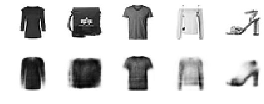
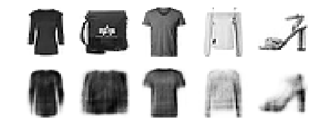
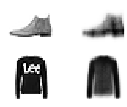
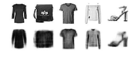
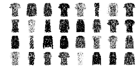
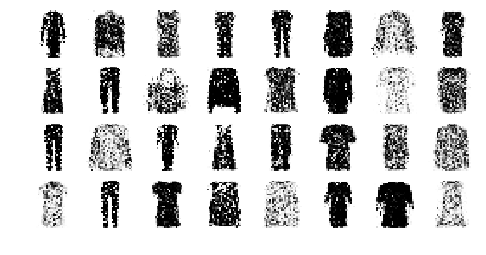
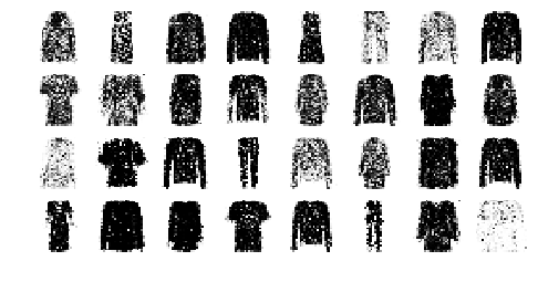
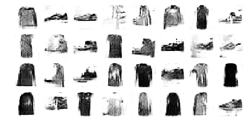
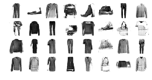
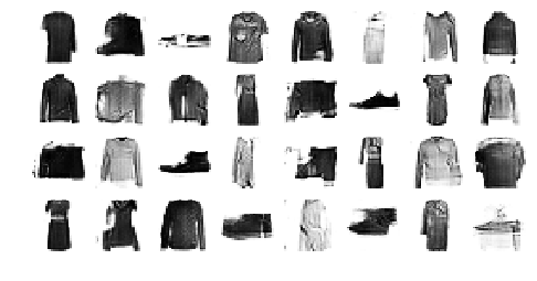
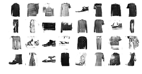
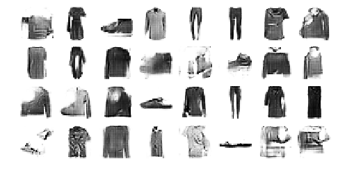
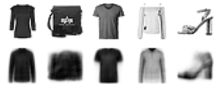
This function processes a few test images through the autoencoder and displays the original images and their reconstructions:
def show_reconstructions(model, images=X_valid, n_images=5):
    reconstructions = model.predict(images[:n_images])
    fig = plt.figure(figsize=(n_images * 1.5, 3))
    for image_index in range(n_images):
        plt.subplot(2, n_images, 1 + image_index)
        plot_image(images[image_index])
        plt.subplot(2, n_images, 1 + n_images + image_index)
        plot_image(reconstructions[image_index])
show_reconstructions(stacked_ae)
save_fig("reconstruction_plot")
Saving figure reconstruction_plot
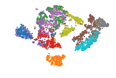
Visualizing Fashion MNIST#
np.random.seed(42)

from sklearn.manifold import TSNE

X_valid_compressed = stacked_encoder.predict(X_valid)
tsne = TSNE()
X_valid_2D = tsne.fit_transform(X_valid_compressed)
X_valid_2D = (X_valid_2D - X_valid_2D.min()) / (X_valid_2D.max() - X_valid_2D.min())
plt.scatter(X_valid_2D[:, 0], X_valid_2D[:, 1], c=y_valid, s=10, cmap="tab10")
plt.axis("off")
plt.show()
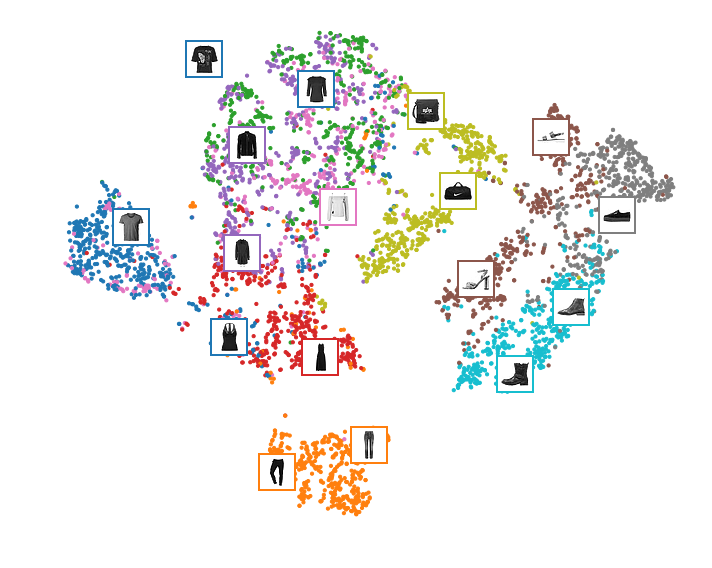
Let’s make this diagram a bit prettier:
# adapted from https://scikit-learn.org/stable/auto_examples/manifold/plot_lle_digits.html
plt.figure(figsize=(10, 8))
cmap = plt.cm.tab10
plt.scatter(X_valid_2D[:, 0], X_valid_2D[:, 1], c=y_valid, s=10, cmap=cmap)
image_positions = np.array([[1., 1.]])
for index, position in enumerate(X_valid_2D):
    dist = np.sum((position - image_positions) ** 2, axis=1)
    if np.min(dist) > 0.02: # if far enough from other images
        image_positions = np.r_[image_positions, [position]]
        imagebox = mpl.offsetbox.AnnotationBbox(
            mpl.offsetbox.OffsetImage(X_valid[index], cmap="binary"),
            position, bboxprops={"edgecolor": cmap(y_valid[index]), "lw": 2})
        plt.gca().add_artist(imagebox)
plt.axis("off")
save_fig("fashion_mnist_visualization_plot")
plt.show()
Saving figure fashion_mnist_visualization_plot
Tying weights#
It is common to tie the weights of the encoder and the decoder, by simply using the transpose of the encoder’s weights as the decoder weights. For this, we need to use a custom layer.
class DenseTranspose(keras.layers.Layer):
    def __init__(self, dense, activation=None, **kwargs):
        self.dense = dense
        self.activation = keras.activations.get(activation)
        super().__init__(**kwargs)
    def build(self, batch_input_shape):
        self.biases = self.add_weight(name="bias",
                                      shape=[self.dense.input_shape[-1]],
                                      initializer="zeros")
        super().build(batch_input_shape)
    def call(self, inputs):
        z = tf.matmul(inputs, self.dense.weights[0], transpose_b=True)
        return self.activation(z + self.biases)
keras.backend.clear_session()
tf.random.set_seed(42)
np.random.seed(42)

dense_1 = keras.layers.Dense(100, activation="selu")
dense_2 = keras.layers.Dense(30, activation="selu")

tied_encoder = keras.models.Sequential([
    keras.layers.Flatten(input_shape=[28, 28]),
    dense_1,
    dense_2
])

tied_decoder = keras.models.Sequential([
    DenseTranspose(dense_2, activation="selu"),
    DenseTranspose(dense_1, activation="sigmoid"),
    keras.layers.Reshape([28, 28])
])

tied_ae = keras.models.Sequential([tied_encoder, tied_decoder])

tied_ae.compile(loss="binary_crossentropy",
                optimizer=keras.optimizers.SGD(learning_rate=1.5), metrics=[rounded_accuracy])
history = tied_ae.fit(X_train, X_train, epochs=10,
                      validation_data=(X_valid, X_valid))
Train on 55000 samples, validate on 5000 samples
Epoch 1/10
55000/55000 [==============================] - 4s 80us/sample - loss: 0.3213 - rounded_accuracy: 0.8996 - val_loss: 0.3038 - val_rounded_accuracy: 0.9154
Epoch 2/10
55000/55000 [==============================] - 4s 74us/sample - loss: 0.2967 - rounded_accuracy: 0.9216 - val_loss: 0.2931 - val_rounded_accuracy: 0.9268
Epoch 3/10
55000/55000 [==============================] - 4s 70us/sample - loss: 0.2916 - rounded_accuracy: 0.9263 - val_loss: 0.2929 - val_rounded_accuracy: 0.9254
Epoch 4/10
55000/55000 [==============================] - 4s 64us/sample - loss: 0.2889 - rounded_accuracy: 0.9287 - val_loss: 0.2905 - val_rounded_accuracy: 0.9316
Epoch 5/10
55000/55000 [==============================] - 4s 70us/sample - loss: 0.2871 - rounded_accuracy: 0.9303 - val_loss: 0.2917 - val_rounded_accuracy: 0.9307
Epoch 6/10
55000/55000 [==============================] - 4s 68us/sample - loss: 0.2858 - rounded_accuracy: 0.9316 - val_loss: 0.2870 - val_rounded_accuracy: 0.9332
Epoch 7/10
55000/55000 [==============================] - 4s 68us/sample - loss: 0.2847 - rounded_accuracy: 0.9327 - val_loss: 0.2865 - val_rounded_accuracy: 0.9336
Epoch 8/10
55000/55000 [==============================] - 4s 71us/sample - loss: 0.2840 - rounded_accuracy: 0.9334 - val_loss: 0.2859 - val_rounded_accuracy: 0.9349
Epoch 9/10
55000/55000 [==============================] - 4s 70us/sample - loss: 0.2834 - rounded_accuracy: 0.9339 - val_loss: 0.2864 - val_rounded_accuracy: 0.9338
Epoch 10/10
55000/55000 [==============================] - 4s 72us/sample - loss: 0.2828 - rounded_accuracy: 0.9345 - val_loss: 0.2839 - val_rounded_accuracy: 0.9338
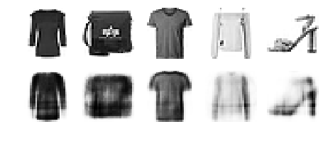
show_reconstructions(tied_ae)
plt.show()
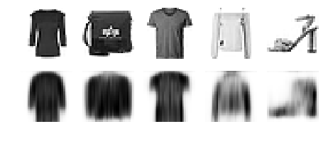
Training one Autoencoder at a Time#
def train_autoencoder(n_neurons, X_train, X_valid, loss, optimizer,
                      n_epochs=10, output_activation=None, metrics=None):
    n_inputs = X_train.shape[-1]
    encoder = keras.models.Sequential([
        keras.layers.Dense(n_neurons, activation="selu", input_shape=[n_inputs])
    ])
    decoder = keras.models.Sequential([
        keras.layers.Dense(n_inputs, activation=output_activation),
    ])
    autoencoder = keras.models.Sequential([encoder, decoder])
    autoencoder.compile(optimizer, loss, metrics=metrics)
    autoencoder.fit(X_train, X_train, epochs=n_epochs,
                    validation_data=(X_valid, X_valid))
    return encoder, decoder, encoder(X_train), encoder(X_valid)
tf.random.set_seed(42)
np.random.seed(42)

K = keras.backend
X_train_flat = K.batch_flatten(X_train) # equivalent to .reshape(-1, 28 * 28)
X_valid_flat = K.batch_flatten(X_valid)
enc1, dec1, X_train_enc1, X_valid_enc1 = train_autoencoder(
    100, X_train_flat, X_valid_flat, "binary_crossentropy",
    keras.optimizers.SGD(learning_rate=1.5), output_activation="sigmoid",
    metrics=[rounded_accuracy])
enc2, dec2, _, _ = train_autoencoder(
    30, X_train_enc1, X_valid_enc1, "mse", keras.optimizers.SGD(learning_rate=0.05),
    output_activation="selu")
Train on 55000 samples, validate on 5000 samples
Epoch 1/10
55000/55000 [==============================] - 4s 73us/sample - loss: 0.3446 - rounded_accuracy: 0.8874 - val_loss: 0.3122 - val_rounded_accuracy: 0.9147
Epoch 2/10
55000/55000 [==============================] - 4s 68us/sample - loss: 0.3039 - rounded_accuracy: 0.9204 - val_loss: 0.3006 - val_rounded_accuracy: 0.9241
Epoch 3/10
55000/55000 [==============================] - 4s 69us/sample - loss: 0.2949 - rounded_accuracy: 0.9286 - val_loss: 0.2933 - val_rounded_accuracy: 0.9319
Epoch 4/10
55000/55000 [==============================] - 4s 68us/sample - loss: 0.2890 - rounded_accuracy: 0.9343 - val_loss: 0.2887 - val_rounded_accuracy: 0.9362
Epoch 5/10
55000/55000 [==============================] - 4s 72us/sample - loss: 0.2853 - rounded_accuracy: 0.9379 - val_loss: 0.2856 - val_rounded_accuracy: 0.9390
Epoch 6/10
55000/55000 [==============================] - 4s 67us/sample - loss: 0.2826 - rounded_accuracy: 0.9404 - val_loss: 0.2833 - val_rounded_accuracy: 0.9410
Epoch 7/10
55000/55000 [==============================] - 4s 69us/sample - loss: 0.2806 - rounded_accuracy: 0.9424 - val_loss: 0.2816 - val_rounded_accuracy: 0.9430
Epoch 8/10
55000/55000 [==============================] - 4s 68us/sample - loss: 0.2791 - rounded_accuracy: 0.9439 - val_loss: 0.2802 - val_rounded_accuracy: 0.9448
Epoch 9/10
55000/55000 [==============================] - 4s 68us/sample - loss: 0.2778 - rounded_accuracy: 0.9451 - val_loss: 0.2790 - val_rounded_accuracy: 0.9454
Epoch 10/10
55000/55000 [==============================] - 4s 65us/sample - loss: 0.2768 - rounded_accuracy: 0.9461 - val_loss: 0.2781 - val_rounded_accuracy: 0.9462
Train on 55000 samples, validate on 5000 samples
Epoch 1/10
55000/55000 [==============================] - 2s 35us/sample - loss: 0.5678 - val_loss: 0.2887
Epoch 2/10
55000/55000 [==============================] - 2s 30us/sample - loss: 0.2633 - val_loss: 0.2512
Epoch 3/10
55000/55000 [==============================] - 2s 33us/sample - loss: 0.2237 - val_loss: 0.2115
Epoch 4/10
55000/55000 [==============================] - 2s 33us/sample - loss: 0.2025 - val_loss: 0.1967
Epoch 5/10
55000/55000 [==============================] - 2s 31us/sample - loss: 0.1909 - val_loss: 0.1864
Epoch 6/10
55000/55000 [==============================] - 2s 29us/sample - loss: 0.1824 - val_loss: 0.1734
Epoch 7/10
55000/55000 [==============================] - 2s 31us/sample - loss: 0.1750 - val_loss: 0.1696
Epoch 8/10
55000/55000 [==============================] - 2s 31us/sample - loss: 0.1732 - val_loss: 0.1719
Epoch 9/10
55000/55000 [==============================] - 2s 30us/sample - loss: 0.1711 - val_loss: 0.1917
Epoch 10/10
55000/55000 [==============================] - 2s 29us/sample - loss: 0.1704 - val_loss: 0.1687
stacked_ae_1_by_1 = keras.models.Sequential([
    keras.layers.Flatten(input_shape=[28, 28]),
    enc1, enc2, dec2, dec1,
    keras.layers.Reshape([28, 28])
])
show_reconstructions(stacked_ae_1_by_1)
plt.show()
stacked_ae_1_by_1.compile(loss="binary_crossentropy",
                          optimizer=keras.optimizers.SGD(learning_rate=0.1), metrics=[rounded_accuracy])
history = stacked_ae_1_by_1.fit(X_train, X_train, epochs=10,
                                validation_data=(X_valid, X_valid))
Train on 55000 samples, validate on 5000 samples
Epoch 1/10
55000/55000 [==============================] - 5s 83us/sample - loss: 0.2853 - rounded_accuracy: 0.9359 - val_loss: 0.2868 - val_rounded_accuracy: 0.9361
Epoch 2/10
55000/55000 [==============================] - 4s 70us/sample - loss: 0.2849 - rounded_accuracy: 0.9363 - val_loss: 0.2866 - val_rounded_accuracy: 0.9364
Epoch 3/10
55000/55000 [==============================] - 4s 66us/sample - loss: 0.2847 - rounded_accuracy: 0.9365 - val_loss: 0.2864 - val_rounded_accuracy: 0.9362
Epoch 4/10
55000/55000 [==============================] - 4s 76us/sample - loss: 0.2846 - rounded_accuracy: 0.9366 - val_loss: 0.2863 - val_rounded_accuracy: 0.9367
Epoch 5/10
55000/55000 [==============================] - 4s 74us/sample - loss: 0.2844 - rounded_accuracy: 0.9368 - val_loss: 0.2862 - val_rounded_accuracy: 0.9369
Epoch 6/10
55000/55000 [==============================] - 4s 66us/sample - loss: 0.2843 - rounded_accuracy: 0.9369 - val_loss: 0.2861 - val_rounded_accuracy: 0.9368
Epoch 7/10
55000/55000 [==============================] - 4s 67us/sample - loss: 0.2842 - rounded_accuracy: 0.9370 - val_loss: 0.2860 - val_rounded_accuracy: 0.9368
Epoch 8/10
55000/55000 [==============================] - 4s 66us/sample - loss: 0.2841 - rounded_accuracy: 0.9371 - val_loss: 0.2859 - val_rounded_accuracy: 0.9369
Epoch 9/10
55000/55000 [==============================] - 4s 67us/sample - loss: 0.2840 - rounded_accuracy: 0.9372 - val_loss: 0.2858 - val_rounded_accuracy: 0.9368
Epoch 10/10
55000/55000 [==============================] - 4s 66us/sample - loss: 0.2839 - rounded_accuracy: 0.9373 - val_loss: 0.2857 - val_rounded_accuracy: 0.9371
show_reconstructions(stacked_ae_1_by_1)
plt.show()

Using Convolutional Layers Instead of Dense Layers#
Let’s build a stacked Autoencoder with 3 hidden layers and 1 output layer (i.e., 2 stacked Autoencoders).
tf.random.set_seed(42)
np.random.seed(42)

conv_encoder = keras.models.Sequential([
    keras.layers.Reshape([28, 28, 1], input_shape=[28, 28]),
    keras.layers.Conv2D(16, kernel_size=3, padding="SAME", activation="selu"),
    keras.layers.MaxPool2D(pool_size=2),
    keras.layers.Conv2D(32, kernel_size=3, padding="SAME", activation="selu"),
    keras.layers.MaxPool2D(pool_size=2),
    keras.layers.Conv2D(64, kernel_size=3, padding="SAME", activation="selu"),
    keras.layers.MaxPool2D(pool_size=2)
])
conv_decoder = keras.models.Sequential([
    keras.layers.Conv2DTranspose(32, kernel_size=3, strides=2, padding="VALID", activation="selu",
                                 input_shape=[3, 3, 64]),
    keras.layers.Conv2DTranspose(16, kernel_size=3, strides=2, padding="SAME", activation="selu"),
    keras.layers.Conv2DTranspose(1, kernel_size=3, strides=2, padding="SAME", activation="sigmoid"),
    keras.layers.Reshape([28, 28])
])
conv_ae = keras.models.Sequential([conv_encoder, conv_decoder])

conv_ae.compile(loss="binary_crossentropy", optimizer=keras.optimizers.SGD(learning_rate=1.0),
                metrics=[rounded_accuracy])
history = conv_ae.fit(X_train, X_train, epochs=5,
                      validation_data=(X_valid, X_valid))
Train on 55000 samples, validate on 5000 samples
Epoch 1/5
55000/55000 [==============================] - 40s 734us/sample - loss: 0.3017 - accuracy: 0.5064 - val_loss: 0.2842 - val_accuracy: 0.5058
Epoch 2/5
55000/55000 [==============================] - 39s 712us/sample - loss: 0.2756 - accuracy: 0.5088 - val_loss: 0.2739 - val_accuracy: 0.5058
Epoch 3/5
55000/55000 [==============================] - 39s 715us/sample - loss: 0.2709 - accuracy: 0.5092 - val_loss: 0.2720 - val_accuracy: 0.5059
Epoch 4/5
55000/55000 [==============================] - 39s 707us/sample - loss: 0.2682 - accuracy: 0.5094 - val_loss: 0.2685 - val_accuracy: 0.5063
Epoch 5/5
55000/55000 [==============================] - 39s 706us/sample - loss: 0.2665 - accuracy: 0.5095 - val_loss: 0.2671 - val_accuracy: 0.5066
conv_encoder.summary()
conv_decoder.summary()
Model: "sequential_16"
_________________________________________________________________
Layer (type)                 Output Shape              Param #
=================================================================
reshape_3 (Reshape)          (None, 28, 28, 1)         0
_________________________________________________________________
conv2d (Conv2D)              (None, 28, 28, 16)        160
_________________________________________________________________
max_pooling2d (MaxPooling2D) (None, 14, 14, 16)        0
_________________________________________________________________
conv2d_1 (Conv2D)            (None, 14, 14, 32)        4640
_________________________________________________________________
max_pooling2d_1 (MaxPooling2 (None, 7, 7, 32)          0
_________________________________________________________________
conv2d_2 (Conv2D)            (None, 7, 7, 64)          18496
_________________________________________________________________
max_pooling2d_2 (MaxPooling2 (None, 3, 3, 64)          0
=================================================================
Total params: 23,296
Trainable params: 23,296
Non-trainable params: 0
_________________________________________________________________
Model: "sequential_17"
_________________________________________________________________
Layer (type)                 Output Shape              Param #
=================================================================
conv2d_transpose (Conv2DTran (None, 7, 7, 32)          18464
_________________________________________________________________
conv2d_transpose_1 (Conv2DTr (None, 14, 14, 16)        4624
_________________________________________________________________
conv2d_transpose_2 (Conv2DTr (None, 28, 28, 1)         145
_________________________________________________________________
reshape_4 (Reshape)          (None, 28, 28)            0
=================================================================
Total params: 23,233
Trainable params: 23,233
Non-trainable params: 0
_________________________________________________________________
show_reconstructions(conv_ae)
plt.show()
Recurrent Autoencoders#
recurrent_encoder = keras.models.Sequential([
    keras.layers.LSTM(100, return_sequences=True, input_shape=[28, 28]),
    keras.layers.LSTM(30)
])
recurrent_decoder = keras.models.Sequential([
    keras.layers.RepeatVector(28, input_shape=[30]),
    keras.layers.LSTM(100, return_sequences=True),
    keras.layers.TimeDistributed(keras.layers.Dense(28, activation="sigmoid"))
])
recurrent_ae = keras.models.Sequential([recurrent_encoder, recurrent_decoder])
recurrent_ae.compile(loss="binary_crossentropy", optimizer=keras.optimizers.SGD(0.1),
                     metrics=[rounded_accuracy])
history = recurrent_ae.fit(X_train, X_train, epochs=10, validation_data=(X_valid, X_valid))
Train on 55000 samples, validate on 5000 samples
Epoch 1/10
55000/55000 [==============================] - 79s 1ms/sample - loss: 0.5165 - rounded_accuracy: 0.7363 - val_loss: 0.4489 - val_rounded_accuracy: 0.8137
Epoch 2/10
55000/55000 [==============================] - 78s 1ms/sample - loss: 0.4049 - rounded_accuracy: 0.8415 - val_loss: 0.3762 - val_rounded_accuracy: 0.8650
Epoch 3/10
55000/55000 [==============================] - 80s 1ms/sample - loss: 0.3662 - rounded_accuracy: 0.8703 - val_loss: 0.3626 - val_rounded_accuracy: 0.8730
Epoch 4/10
55000/55000 [==============================] - 80s 1ms/sample - loss: 0.3505 - rounded_accuracy: 0.8808 - val_loss: 0.3483 - val_rounded_accuracy: 0.8838
Epoch 5/10
55000/55000 [==============================] - 82s 1ms/sample - loss: 0.3398 - rounded_accuracy: 0.8881 - val_loss: 0.3345 - val_rounded_accuracy: 0.8941
Epoch 6/10
55000/55000 [==============================] - 93s 2ms/sample - loss: 0.3328 - rounded_accuracy: 0.8930 - val_loss: 0.3372 - val_rounded_accuracy: 0.8914
Epoch 7/10
55000/55000 [==============================] - 94s 2ms/sample - loss: 0.3280 - rounded_accuracy: 0.8962 - val_loss: 0.3261 - val_rounded_accuracy: 0.8980
Epoch 8/10
55000/55000 [==============================] - 95s 2ms/sample - loss: 0.3244 - rounded_accuracy: 0.8988 - val_loss: 0.3226 - val_rounded_accuracy: 0.9030
Epoch 9/10
55000/55000 [==============================] - 92s 2ms/sample - loss: 0.3215 - rounded_accuracy: 0.9010 - val_loss: 0.3239 - val_rounded_accuracy: 0.8958
Epoch 10/10
55000/55000 [==============================] - 90s 2ms/sample - loss: 0.3190 - rounded_accuracy: 0.9030 - val_loss: 0.3206 - val_rounded_accuracy: 0.9015
<tensorflow.python.keras.callbacks.History at 0x1a5b98fa20>
show_reconstructions(recurrent_ae)
plt.show()
Stacked denoising Autoencoder#
Using Gaussian noise:
tf.random.set_seed(42)
np.random.seed(42)

denoising_encoder = keras.models.Sequential([
    keras.layers.Flatten(input_shape=[28, 28]),
    keras.layers.GaussianNoise(0.2),
    keras.layers.Dense(100, activation="selu"),
    keras.layers.Dense(30, activation="selu")
])
denoising_decoder = keras.models.Sequential([
    keras.layers.Dense(100, activation="selu", input_shape=[30]),
    keras.layers.Dense(28 * 28, activation="sigmoid"),
    keras.layers.Reshape([28, 28])
])
denoising_ae = keras.models.Sequential([denoising_encoder, denoising_decoder])
denoising_ae.compile(loss="binary_crossentropy", optimizer=keras.optimizers.SGD(learning_rate=1.0),
                     metrics=[rounded_accuracy])
history = denoising_ae.fit(X_train, X_train, epochs=10,
                           validation_data=(X_valid, X_valid))
Train on 55000 samples, validate on 5000 samples
Epoch 1/10
55000/55000 [==============================] - 5s 82us/sample - loss: 0.3508 - rounded_accuracy: 0.8768 - val_loss: 0.3231 - val_rounded_accuracy: 0.9065
Epoch 2/10
55000/55000 [==============================] - 4s 75us/sample - loss: 0.3125 - rounded_accuracy: 0.9093 - val_loss: 0.3077 - val_rounded_accuracy: 0.9153
Epoch 3/10
55000/55000 [==============================] - 4s 74us/sample - loss: 0.3061 - rounded_accuracy: 0.9149 - val_loss: 0.3034 - val_rounded_accuracy: 0.9190
Epoch 4/10
55000/55000 [==============================] - 4s 75us/sample - loss: 0.3025 - rounded_accuracy: 0.9181 - val_loss: 0.3007 - val_rounded_accuracy: 0.9195
Epoch 5/10
55000/55000 [==============================] - 4s 75us/sample - loss: 0.2998 - rounded_accuracy: 0.9203 - val_loss: 0.2980 - val_rounded_accuracy: 0.9230
Epoch 6/10
55000/55000 [==============================] - 4s 78us/sample - loss: 0.2979 - rounded_accuracy: 0.9220 - val_loss: 0.2987 - val_rounded_accuracy: 0.9193
Epoch 7/10
55000/55000 [==============================] - 4s 74us/sample - loss: 0.2965 - rounded_accuracy: 0.9233 - val_loss: 0.2945 - val_rounded_accuracy: 0.9269
Epoch 8/10
55000/55000 [==============================] - 4s 75us/sample - loss: 0.2953 - rounded_accuracy: 0.9243 - val_loss: 0.2946 - val_rounded_accuracy: 0.9286
Epoch 9/10
55000/55000 [==============================] - 4s 75us/sample - loss: 0.2943 - rounded_accuracy: 0.9251 - val_loss: 0.2927 - val_rounded_accuracy: 0.9283
Epoch 10/10
55000/55000 [==============================] - 4s 77us/sample - loss: 0.2935 - rounded_accuracy: 0.9258 - val_loss: 0.2920 - val_rounded_accuracy: 0.9291
tf.random.set_seed(42)
np.random.seed(42)

noise = keras.layers.GaussianNoise(0.2)
show_reconstructions(denoising_ae, noise(X_valid, training=True))
plt.show()
Using dropout:
tf.random.set_seed(42)
np.random.seed(42)

dropout_encoder = keras.models.Sequential([
    keras.layers.Flatten(input_shape=[28, 28]),
    keras.layers.Dropout(0.5),
    keras.layers.Dense(100, activation="selu"),
    keras.layers.Dense(30, activation="selu")
])
dropout_decoder = keras.models.Sequential([
    keras.layers.Dense(100, activation="selu", input_shape=[30]),
    keras.layers.Dense(28 * 28, activation="sigmoid"),
    keras.layers.Reshape([28, 28])
])
dropout_ae = keras.models.Sequential([dropout_encoder, dropout_decoder])
dropout_ae.compile(loss="binary_crossentropy", optimizer=keras.optimizers.SGD(learning_rate=1.0),
                   metrics=[rounded_accuracy])
history = dropout_ae.fit(X_train, X_train, epochs=10,
                         validation_data=(X_valid, X_valid))
Train on 55000 samples, validate on 5000 samples
Epoch 1/10
55000/55000 [==============================] - 5s 83us/sample - loss: 0.3564 - accuracy: 0.4969 - val_loss: 0.3206 - val_accuracy: 0.5011
Epoch 2/10
55000/55000 [==============================] - 4s 73us/sample - loss: 0.3182 - accuracy: 0.5034 - val_loss: 0.3113 - val_accuracy: 0.5014
Epoch 3/10
55000/55000 [==============================] - 4s 74us/sample - loss: 0.3130 - accuracy: 0.5042 - val_loss: 0.3079 - val_accuracy: 0.5012
Epoch 4/10
55000/55000 [==============================] - 4s 73us/sample - loss: 0.3091 - accuracy: 0.5048 - val_loss: 0.3037 - val_accuracy: 0.5026
Epoch 5/10
55000/55000 [==============================] - 4s 76us/sample - loss: 0.3066 - accuracy: 0.5052 - val_loss: 0.3032 - val_accuracy: 0.5016
Epoch 6/10
55000/55000 [==============================] - 4s 78us/sample - loss: 0.3047 - accuracy: 0.5054 - val_loss: 0.3001 - val_accuracy: 0.5032
Epoch 7/10
55000/55000 [==============================] - 4s 79us/sample - loss: 0.3033 - accuracy: 0.5056 - val_loss: 0.2987 - val_accuracy: 0.5033
Epoch 8/10
55000/55000 [==============================] - 4s 76us/sample - loss: 0.3021 - accuracy: 0.5057 - val_loss: 0.2976 - val_accuracy: 0.5033
Epoch 9/10
55000/55000 [==============================] - 4s 75us/sample - loss: 0.3012 - accuracy: 0.5058 - val_loss: 0.2976 - val_accuracy: 0.5033
Epoch 10/10
55000/55000 [==============================] - 4s 76us/sample - loss: 0.3004 - accuracy: 0.5059 - val_loss: 0.2958 - val_accuracy: 0.5033
tf.random.set_seed(42)
np.random.seed(42)

dropout = keras.layers.Dropout(0.5)
show_reconstructions(dropout_ae, dropout(X_valid, training=True))
save_fig("dropout_denoising_plot", tight_layout=False)
Saving figure dropout_denoising_plot
Sparse Autoencoder#
Let’s build a simple stacked autoencoder, so we can compare it to the sparse autoencoders we will build. This time we will use the sigmoid activation function for the coding layer, to ensure that the coding values range from 0 to 1:
tf.random.set_seed(42)
np.random.seed(42)

simple_encoder = keras.models.Sequential([
    keras.layers.Flatten(input_shape=[28, 28]),
    keras.layers.Dense(100, activation="selu"),
    keras.layers.Dense(30, activation="sigmoid"),
])
simple_decoder = keras.models.Sequential([
    keras.layers.Dense(100, activation="selu", input_shape=[30]),
    keras.layers.Dense(28 * 28, activation="sigmoid"),
    keras.layers.Reshape([28, 28])
])
simple_ae = keras.models.Sequential([simple_encoder, simple_decoder])
simple_ae.compile(loss="binary_crossentropy", optimizer=keras.optimizers.SGD(learning_rate=1.),
                  metrics=[rounded_accuracy])
history = simple_ae.fit(X_train, X_train, epochs=10,
                        validation_data=(X_valid, X_valid))
Train on 55000 samples, validate on 5000 samples
Epoch 1/10
55000/55000 [==============================] - 4s 78us/sample - loss: 0.4331 - accuracy: 0.4906 - val_loss: 0.3778 - val_accuracy: 0.4911
Epoch 2/10
55000/55000 [==============================] - 4s 67us/sample - loss: 0.3610 - accuracy: 0.4976 - val_loss: 0.3510 - val_accuracy: 0.4972
Epoch 3/10
55000/55000 [==============================] - 4s 68us/sample - loss: 0.3405 - accuracy: 0.5006 - val_loss: 0.3359 - val_accuracy: 0.4990
Epoch 4/10
55000/55000 [==============================] - 4s 68us/sample - loss: 0.3276 - accuracy: 0.5027 - val_loss: 0.3248 - val_accuracy: 0.5003
Epoch 5/10
55000/55000 [==============================] - 4s 72us/sample - loss: 0.3206 - accuracy: 0.5035 - val_loss: 0.3206 - val_accuracy: 0.5007
Epoch 6/10
55000/55000 [==============================] - 4s 68us/sample - loss: 0.3172 - accuracy: 0.5038 - val_loss: 0.3176 - val_accuracy: 0.5010
Epoch 7/10
55000/55000 [==============================] - 4s 68us/sample - loss: 0.3149 - accuracy: 0.5041 - val_loss: 0.3154 - val_accuracy: 0.5013
Epoch 8/10
55000/55000 [==============================] - 4s 69us/sample - loss: 0.3128 - accuracy: 0.5045 - val_loss: 0.3133 - val_accuracy: 0.5014
Epoch 9/10
55000/55000 [==============================] - 4s 68us/sample - loss: 0.3108 - accuracy: 0.5049 - val_loss: 0.3118 - val_accuracy: 0.5023
Epoch 10/10
55000/55000 [==============================] - 4s 71us/sample - loss: 0.3088 - accuracy: 0.5053 - val_loss: 0.3092 - val_accuracy: 0.5023
show_reconstructions(simple_ae)
plt.show()
Let’s create a couple functions to print nice activation histograms:
def plot_percent_hist(ax, data, bins):
    counts, _ = np.histogram(data, bins=bins)
    widths = bins[1:] - bins[:-1]
    x = bins[:-1] + widths / 2
    ax.bar(x, counts / len(data), width=widths*0.8)
    ax.xaxis.set_ticks(bins)
    ax.yaxis.set_major_formatter(mpl.ticker.FuncFormatter(
        lambda y, position: "{}%".format(int(np.round(100 * y)))))
    ax.grid(True)
def plot_activations_histogram(encoder, height=1, n_bins=10):
    X_valid_codings = encoder(X_valid).numpy()
    activation_means = X_valid_codings.mean(axis=0)
    mean = activation_means.mean()
    bins = np.linspace(0, 1, n_bins + 1)

    fig, [ax1, ax2] = plt.subplots(figsize=(10, 3), nrows=1, ncols=2, sharey=True)
    plot_percent_hist(ax1, X_valid_codings.ravel(), bins)
    ax1.plot([mean, mean], [0, height], "k--", label="Overall Mean = {:.2f}".format(mean))
    ax1.legend(loc="upper center", fontsize=14)
    ax1.set_xlabel("Activation")
    ax1.set_ylabel("% Activations")
    ax1.axis([0, 1, 0, height])
    plot_percent_hist(ax2, activation_means, bins)
    ax2.plot([mean, mean], [0, height], "k--")
    ax2.set_xlabel("Neuron Mean Activation")
    ax2.set_ylabel("% Neurons")
    ax2.axis([0, 1, 0, height])
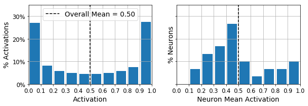
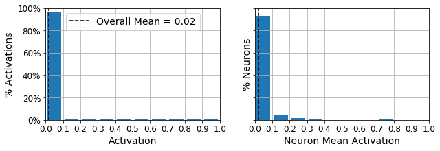
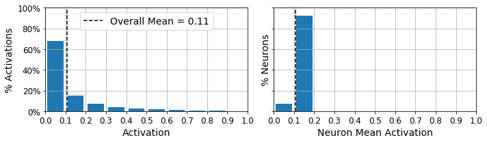
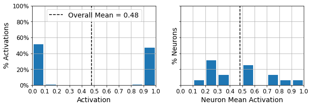
Let’s use these functions to plot histograms of the activations of the encoding layer. The histogram on the left shows the distribution of all the activations. You can see that values close to 0 or 1 are more frequent overall, which is consistent with the saturating nature of the sigmoid function. The histogram on the right shows the distribution of mean neuron activations: you can see that most neurons have a mean activation close to 0.5. Both histograms tell us that each neuron tends to either fire close to 0 or 1, with about 50% probability each. However, some neurons fire almost all the time (right side of the right histogram).
plot_activations_histogram(simple_encoder, height=0.35)
plt.show()
Now let’s add \(\ell_1\) regularization to the coding layer:
tf.random.set_seed(42)
np.random.seed(42)

sparse_l1_encoder = keras.models.Sequential([
    keras.layers.Flatten(input_shape=[28, 28]),
    keras.layers.Dense(100, activation="selu"),
    keras.layers.Dense(300, activation="sigmoid"),
    keras.layers.ActivityRegularization(l1=1e-3)  # Alternatively, you could add
                                                  # activity_regularizer=keras.regularizers.l1(1e-3)
                                                  # to the previous layer.
])
sparse_l1_decoder = keras.models.Sequential([
    keras.layers.Dense(100, activation="selu", input_shape=[300]),
    keras.layers.Dense(28 * 28, activation="sigmoid"),
    keras.layers.Reshape([28, 28])
])
sparse_l1_ae = keras.models.Sequential([sparse_l1_encoder, sparse_l1_decoder])
sparse_l1_ae.compile(loss="binary_crossentropy", optimizer=keras.optimizers.SGD(learning_rate=1.0),
                     metrics=[rounded_accuracy])
history = sparse_l1_ae.fit(X_train, X_train, epochs=10,
                           validation_data=(X_valid, X_valid))
Train on 55000 samples, validate on 5000 samples
Epoch 1/10
55000/55000 [==============================] - 5s 98us/sample - loss: 0.4306 - accuracy: 0.4947 - val_loss: 0.3819 - val_accuracy: 0.4897
Epoch 2/10
55000/55000 [==============================] - 4s 75us/sample - loss: 0.3689 - accuracy: 0.4971 - val_loss: 0.3639 - val_accuracy: 0.4940
Epoch 3/10
55000/55000 [==============================] - 5s 86us/sample - loss: 0.3553 - accuracy: 0.4987 - val_loss: 0.3513 - val_accuracy: 0.4970
Epoch 4/10
55000/55000 [==============================] - 4s 78us/sample - loss: 0.3443 - accuracy: 0.5003 - val_loss: 0.3428 - val_accuracy: 0.4964
Epoch 5/10
55000/55000 [==============================] - 4s 76us/sample - loss: 0.3379 - accuracy: 0.5009 - val_loss: 0.3372 - val_accuracy: 0.4979
Epoch 6/10
55000/55000 [==============================] - 4s 76us/sample - loss: 0.3332 - accuracy: 0.5015 - val_loss: 0.3329 - val_accuracy: 0.4980
Epoch 7/10
55000/55000 [==============================] - 4s 78us/sample - loss: 0.3286 - accuracy: 0.5025 - val_loss: 0.3306 - val_accuracy: 0.4981
Epoch 8/10
55000/55000 [==============================] - 4s 76us/sample - loss: 0.3249 - accuracy: 0.5032 - val_loss: 0.3254 - val_accuracy: 0.5000
Epoch 9/10
55000/55000 [==============================] - 4s 80us/sample - loss: 0.3223 - accuracy: 0.5036 - val_loss: 0.3244 - val_accuracy: 0.4995
Epoch 10/10
55000/55000 [==============================] - 4s 75us/sample - loss: 0.3205 - accuracy: 0.5039 - val_loss: 0.3212 - val_accuracy: 0.5014
show_reconstructions(sparse_l1_ae)
plot_activations_histogram(sparse_l1_encoder, height=1.)
plt.show()
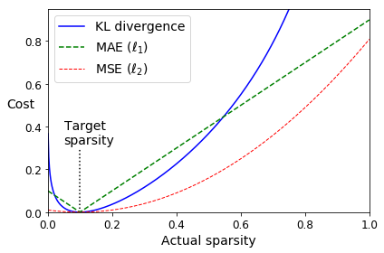
Let’s use the KL Divergence loss instead to ensure sparsity, and target 10% sparsity rather than 0%:
p = 0.1
q = np.linspace(0.001, 0.999, 500)
kl_div = p * np.log(p / q) + (1 - p) * np.log((1 - p) / (1 - q))
mse = (p - q)**2
mae = np.abs(p - q)
plt.plot([p, p], [0, 0.3], "k:")
plt.text(0.05, 0.32, "Target\nsparsity", fontsize=14)
plt.plot(q, kl_div, "b-", label="KL divergence")
plt.plot(q, mae, "g--", label=r"MAE ($\ell_1$)")
plt.plot(q, mse, "r--", linewidth=1, label=r"MSE ($\ell_2$)")
plt.legend(loc="upper left", fontsize=14)
plt.xlabel("Actual sparsity")
plt.ylabel("Cost", rotation=0)
plt.axis([0, 1, 0, 0.95])
save_fig("sparsity_loss_plot")
Saving figure sparsity_loss_plot
K = keras.backend
kl_divergence = keras.losses.kullback_leibler_divergence

class KLDivergenceRegularizer(keras.regularizers.Regularizer):
    def __init__(self, weight, target=0.1):
        self.weight = weight
        self.target = target
    def __call__(self, inputs):
        mean_activities = K.mean(inputs, axis=0)
        return self.weight * (
            kl_divergence(self.target, mean_activities) +
            kl_divergence(1. - self.target, 1. - mean_activities))
tf.random.set_seed(42)
np.random.seed(42)

kld_reg = KLDivergenceRegularizer(weight=0.05, target=0.1)
sparse_kl_encoder = keras.models.Sequential([
    keras.layers.Flatten(input_shape=[28, 28]),
    keras.layers.Dense(100, activation="selu"),
    keras.layers.Dense(300, activation="sigmoid", activity_regularizer=kld_reg)
])
sparse_kl_decoder = keras.models.Sequential([
    keras.layers.Dense(100, activation="selu", input_shape=[300]),
    keras.layers.Dense(28 * 28, activation="sigmoid"),
    keras.layers.Reshape([28, 28])
])
sparse_kl_ae = keras.models.Sequential([sparse_kl_encoder, sparse_kl_decoder])
sparse_kl_ae.compile(loss="binary_crossentropy", optimizer=keras.optimizers.SGD(learning_rate=1.0),
              metrics=[rounded_accuracy])
history = sparse_kl_ae.fit(X_train, X_train, epochs=10,
                           validation_data=(X_valid, X_valid))
Train on 55000 samples, validate on 5000 samples
Epoch 1/10
55000/55000 [==============================] - 6s 103us/sample - loss: 0.4151 - rounded_accuracy: 0.8121 - val_loss: 0.3714 - val_rounded_accuracy: 0.8560
Epoch 2/10
55000/55000 [==============================] - 4s 81us/sample - loss: 0.3532 - rounded_accuracy: 0.8762 - val_loss: 0.3442 - val_rounded_accuracy: 0.8842
Epoch 3/10
55000/55000 [==============================] - 5s 83us/sample - loss: 0.3340 - rounded_accuracy: 0.8919 - val_loss: 0.3292 - val_rounded_accuracy: 0.8976
Epoch 4/10
55000/55000 [==============================] - 5s 84us/sample - loss: 0.3224 - rounded_accuracy: 0.9018 - val_loss: 0.3213 - val_rounded_accuracy: 0.9040
Epoch 5/10
55000/55000 [==============================] - 5s 85us/sample - loss: 0.3170 - rounded_accuracy: 0.9062 - val_loss: 0.3170 - val_rounded_accuracy: 0.9075
Epoch 6/10
55000/55000 [==============================] - 5s 82us/sample - loss: 0.3134 - rounded_accuracy: 0.9093 - val_loss: 0.3140 - val_rounded_accuracy: 0.9105
Epoch 7/10
55000/55000 [==============================] - 5s 85us/sample - loss: 0.3107 - rounded_accuracy: 0.9116 - val_loss: 0.3114 - val_rounded_accuracy: 0.9121
Epoch 8/10
55000/55000 [==============================] - 5s 83us/sample - loss: 0.3084 - rounded_accuracy: 0.9136 - val_loss: 0.3094 - val_rounded_accuracy: 0.9145
Epoch 9/10
55000/55000 [==============================] - 5s 83us/sample - loss: 0.3064 - rounded_accuracy: 0.9154 - val_loss: 0.3074 - val_rounded_accuracy: 0.9166
Epoch 10/10
55000/55000 [==============================] - 5s 84us/sample - loss: 0.3044 - rounded_accuracy: 0.9170 - val_loss: 0.3053 - val_rounded_accuracy: 0.9174
show_reconstructions(sparse_kl_ae)
plot_activations_histogram(sparse_kl_encoder)
save_fig("sparse_autoencoder_plot")
plt.show()
Saving figure sparse_autoencoder_plot
Variational Autoencoder#
class Sampling(keras.layers.Layer):
    def call(self, inputs):
        mean, log_var = inputs
        return K.random_normal(tf.shape(log_var)) * K.exp(log_var / 2) + mean
tf.random.set_seed(42)
np.random.seed(42)

codings_size = 10

inputs = keras.layers.Input(shape=[28, 28])
z = keras.layers.Flatten()(inputs)
z = keras.layers.Dense(150, activation="selu")(z)
z = keras.layers.Dense(100, activation="selu")(z)
codings_mean = keras.layers.Dense(codings_size)(z)
codings_log_var = keras.layers.Dense(codings_size)(z)
codings = Sampling()([codings_mean, codings_log_var])
variational_encoder = keras.models.Model(
    inputs=[inputs], outputs=[codings_mean, codings_log_var, codings])

decoder_inputs = keras.layers.Input(shape=[codings_size])
x = keras.layers.Dense(100, activation="selu")(decoder_inputs)
x = keras.layers.Dense(150, activation="selu")(x)
x = keras.layers.Dense(28 * 28, activation="sigmoid")(x)
outputs = keras.layers.Reshape([28, 28])(x)
variational_decoder = keras.models.Model(inputs=[decoder_inputs], outputs=[outputs])

_, _, codings = variational_encoder(inputs)
reconstructions = variational_decoder(codings)
variational_ae = keras.models.Model(inputs=[inputs], outputs=[reconstructions])

latent_loss = -0.5 * K.sum(
    1 + codings_log_var - K.exp(codings_log_var) - K.square(codings_mean),
    axis=-1)
variational_ae.add_loss(K.mean(latent_loss) / 784.)
variational_ae.compile(loss="binary_crossentropy", optimizer="rmsprop", metrics=[rounded_accuracy])
history = variational_ae.fit(X_train, X_train, epochs=25, batch_size=128,
                             validation_data=(X_valid, X_valid))
Train on 55000 samples, validate on 5000 samples
Epoch 1/25
55000/55000 [==============================] - 5s 84us/sample - loss: 0.3889 - rounded_accuracy: 0.8608 - val_loss: 0.3592 - val_rounded_accuracy: 0.8840
Epoch 2/25
55000/55000 [==============================] - 3s 60us/sample - loss: 0.3429 - rounded_accuracy: 0.8974 - val_loss: 0.3369 - val_rounded_accuracy: 0.8982
Epoch 3/25
55000/55000 [==============================] - 3s 53us/sample - loss: 0.3329 - rounded_accuracy: 0.9050 - val_loss: 0.3356 - val_rounded_accuracy: 0.9022
Epoch 4/25
55000/55000 [==============================] - 3s 61us/sample - loss: 0.3275 - rounded_accuracy: 0.9092 - val_loss: 0.3255 - val_rounded_accuracy: 0.9105
Epoch 5/25
55000/55000 [==============================] - 3s 59us/sample - loss: 0.3243 - rounded_accuracy: 0.9119 - val_loss: 0.3232 - val_rounded_accuracy: 0.9169
Epoch 6/25
55000/55000 [==============================] - 3s 58us/sample - loss: 0.3219 - rounded_accuracy: 0.9138 - val_loss: 0.3236 - val_rounded_accuracy: 0.9149
Epoch 7/25
55000/55000 [==============================] - 3s 55us/sample - loss: 0.3204 - rounded_accuracy: 0.9150 - val_loss: 0.3194 - val_rounded_accuracy: 0.9176
Epoch 8/25
55000/55000 [==============================] - 3s 56us/sample - loss: 0.3190 - rounded_accuracy: 0.9162 - val_loss: 0.3195 - val_rounded_accuracy: 0.9146
Epoch 9/25
55000/55000 [==============================] - 3s 58us/sample - loss: 0.3180 - rounded_accuracy: 0.9169 - val_loss: 0.3197 - val_rounded_accuracy: 0.9151
Epoch 10/25
55000/55000 [==============================] - 3s 60us/sample - loss: 0.3172 - rounded_accuracy: 0.9178 - val_loss: 0.3169 - val_rounded_accuracy: 0.9192
Epoch 11/25
55000/55000 [==============================] - 3s 57us/sample - loss: 0.3165 - rounded_accuracy: 0.9183 - val_loss: 0.3197 - val_rounded_accuracy: 0.9177
Epoch 12/25
55000/55000 [==============================] - 3s 58us/sample - loss: 0.3159 - rounded_accuracy: 0.9188 - val_loss: 0.3168 - val_rounded_accuracy: 0.9185
Epoch 13/25
55000/55000 [==============================] - 3s 62us/sample - loss: 0.3154 - rounded_accuracy: 0.9193 - val_loss: 0.3175 - val_rounded_accuracy: 0.9178
Epoch 14/25
55000/55000 [==============================] - 4s 64us/sample - loss: 0.3150 - rounded_accuracy: 0.9197 - val_loss: 0.3170 - val_rounded_accuracy: 0.9201
Epoch 15/25
55000/55000 [==============================] - 3s 60us/sample - loss: 0.3145 - rounded_accuracy: 0.9199 - val_loss: 0.3177 - val_rounded_accuracy: 0.9202
Epoch 16/25
55000/55000 [==============================] - 3s 58us/sample - loss: 0.3141 - rounded_accuracy: 0.9202 - val_loss: 0.3161 - val_rounded_accuracy: 0.9206
Epoch 17/25
55000/55000 [==============================] - 3s 61us/sample - loss: 0.3138 - rounded_accuracy: 0.9206 - val_loss: 0.3164 - val_rounded_accuracy: 0.9173
Epoch 18/25
55000/55000 [==============================] - 3s 58us/sample - loss: 0.3135 - rounded_accuracy: 0.9209 - val_loss: 0.3160 - val_rounded_accuracy: 0.9174
Epoch 19/25
55000/55000 [==============================] - 3s 58us/sample - loss: 0.3132 - rounded_accuracy: 0.9211 - val_loss: 0.3160 - val_rounded_accuracy: 0.9216
Epoch 20/25
55000/55000 [==============================] - 3s 61us/sample - loss: 0.3129 - rounded_accuracy: 0.9213 - val_loss: 0.3155 - val_rounded_accuracy: 0.9212
Epoch 21/25
55000/55000 [==============================] - 3s 61us/sample - loss: 0.3127 - rounded_accuracy: 0.9215 - val_loss: 0.3163 - val_rounded_accuracy: 0.9174
Epoch 22/25
55000/55000 [==============================] - 3s 60us/sample - loss: 0.3125 - rounded_accuracy: 0.9217 - val_loss: 0.3145 - val_rounded_accuracy: 0.9215
Epoch 23/25
55000/55000 [==============================] - 3s 53us/sample - loss: 0.3122 - rounded_accuracy: 0.9219 - val_loss: 0.3158 - val_rounded_accuracy: 0.9201
Epoch 24/25
55000/55000 [==============================] - 3s 56us/sample - loss: 0.3121 - rounded_accuracy: 0.9222 - val_loss: 0.3136 - val_rounded_accuracy: 0.9211
Epoch 25/25
55000/55000 [==============================] - 3s 54us/sample - loss: 0.3118 - rounded_accuracy: 0.9223 - val_loss: 0.3133 - val_rounded_accuracy: 0.9228
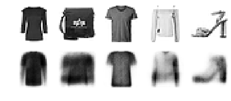
show_reconstructions(variational_ae)
plt.show()
Generate Fashion Images#
def plot_multiple_images(images, n_cols=None):
    n_cols = n_cols or len(images)
    n_rows = (len(images) - 1) // n_cols + 1
    if images.shape[-1] == 1:
        images = np.squeeze(images, axis=-1)
    plt.figure(figsize=(n_cols, n_rows))
    for index, image in enumerate(images):
        plt.subplot(n_rows, n_cols, index + 1)
        plt.imshow(image, cmap="binary")
        plt.axis("off")
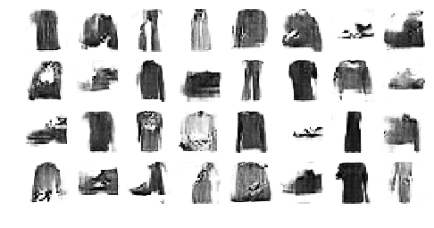
Let’s generate a few random codings, decode them and plot the resulting images:
tf.random.set_seed(42)

codings = tf.random.normal(shape=[12, codings_size])
images = variational_decoder(codings).numpy()
plot_multiple_images(images, 4)
save_fig("vae_generated_images_plot", tight_layout=False)
Saving figure vae_generated_images_plot

Now let’s perform semantic interpolation between these images:
tf.random.set_seed(42)
np.random.seed(42)

codings_grid = tf.reshape(codings, [1, 3, 4, codings_size])
larger_grid = tf.image.resize(codings_grid, size=[5, 7])
interpolated_codings = tf.reshape(larger_grid, [-1, codings_size])
images = variational_decoder(interpolated_codings).numpy()

plt.figure(figsize=(7, 5))
for index, image in enumerate(images):
    plt.subplot(5, 7, index + 1)
    if index%7%2==0 and index//7%2==0:
        plt.gca().get_xaxis().set_visible(False)
        plt.gca().get_yaxis().set_visible(False)
    else:
        plt.axis("off")
    plt.imshow(image, cmap="binary")
save_fig("semantic_interpolation_plot", tight_layout=False)
Saving figure semantic_interpolation_plot
Generative Adversarial Networks#
np.random.seed(42)
tf.random.set_seed(42)

codings_size = 30

generator = keras.models.Sequential([
    keras.layers.Dense(100, activation="selu", input_shape=[codings_size]),
    keras.layers.Dense(150, activation="selu"),
    keras.layers.Dense(28 * 28, activation="sigmoid"),
    keras.layers.Reshape([28, 28])
])
discriminator = keras.models.Sequential([
    keras.layers.Flatten(input_shape=[28, 28]),
    keras.layers.Dense(150, activation="selu"),
    keras.layers.Dense(100, activation="selu"),
    keras.layers.Dense(1, activation="sigmoid")
])
gan = keras.models.Sequential([generator, discriminator])
discriminator.compile(loss="binary_crossentropy", optimizer="rmsprop")
discriminator.trainable = False
gan.compile(loss="binary_crossentropy", optimizer="rmsprop")
batch_size = 32
dataset = tf.data.Dataset.from_tensor_slices(X_train).shuffle(1000)
dataset = dataset.batch(batch_size, drop_remainder=True).prefetch(1)
def train_gan(gan, dataset, batch_size, codings_size, n_epochs=50):
    generator, discriminator = gan.layers
    for epoch in range(n_epochs):
        print("Epoch {}/{}".format(epoch + 1, n_epochs))              # not shown in the book
        for X_batch in dataset:
            # phase 1 - training the discriminator
            noise = tf.random.normal(shape=[batch_size, codings_size])
            generated_images = generator(noise)
            X_fake_and_real = tf.concat([generated_images, X_batch], axis=0)
            y1 = tf.constant([[0.]] * batch_size + [[1.]] * batch_size)
            discriminator.trainable = True
            discriminator.train_on_batch(X_fake_and_real, y1)
            # phase 2 - training the generator
            noise = tf.random.normal(shape=[batch_size, codings_size])
            y2 = tf.constant([[1.]] * batch_size)
            discriminator.trainable = False
            gan.train_on_batch(noise, y2)
        plot_multiple_images(generated_images, 8)                     # not shown
        plt.show()                                                    # not shown
train_gan(gan, dataset, batch_size, codings_size, n_epochs=1)
Epoch 1/1
tf.random.set_seed(42)
np.random.seed(42)

noise = tf.random.normal(shape=[batch_size, codings_size])
generated_images = generator(noise)
plot_multiple_images(generated_images, 8)
save_fig("gan_generated_images_plot", tight_layout=False)
Saving figure gan_generated_images_plot

train_gan(gan, dataset, batch_size, codings_size)
Epoch 1/50
Epoch 2/50
Epoch 3/50
Epoch 4/50

Epoch 5/50
Epoch 6/50
Epoch 7/50
Epoch 8/50
Epoch 9/50
Epoch 10/50
Epoch 11/50
Epoch 12/50
Epoch 13/50
Epoch 14/50
Epoch 15/50
Epoch 16/50
Epoch 17/50
Epoch 18/50
Epoch 19/50
Epoch 20/50
Epoch 21/50

Epoch 22/50

Epoch 23/50
Epoch 24/50
Epoch 25/50
Epoch 26/50

Epoch 27/50
Epoch 28/50
Epoch 29/50
Epoch 30/50
Epoch 31/50
Epoch 32/50
Epoch 33/50
Epoch 34/50
Epoch 35/50
Epoch 36/50
Epoch 37/50
Epoch 38/50
Epoch 39/50
Epoch 40/50
Epoch 41/50
Epoch 42/50
Epoch 43/50
Epoch 44/50
Epoch 45/50
Epoch 46/50
Epoch 47/50
Epoch 48/50
Epoch 49/50
Epoch 50/50
Deep Convolutional GAN#
tf.random.set_seed(42)
np.random.seed(42)

codings_size = 100

generator = keras.models.Sequential([
    keras.layers.Dense(7 * 7 * 128, input_shape=[codings_size]),
    keras.layers.Reshape([7, 7, 128]),
    keras.layers.BatchNormalization(),
    keras.layers.Conv2DTranspose(64, kernel_size=5, strides=2, padding="SAME",
                                 activation="selu"),
    keras.layers.BatchNormalization(),
    keras.layers.Conv2DTranspose(1, kernel_size=5, strides=2, padding="SAME",
                                 activation="tanh"),
])
discriminator = keras.models.Sequential([
    keras.layers.Conv2D(64, kernel_size=5, strides=2, padding="SAME",
                        activation=keras.layers.LeakyReLU(0.2),
                        input_shape=[28, 28, 1]),
    keras.layers.Dropout(0.4),
    keras.layers.Conv2D(128, kernel_size=5, strides=2, padding="SAME",
                        activation=keras.layers.LeakyReLU(0.2)),
    keras.layers.Dropout(0.4),
    keras.layers.Flatten(),
    keras.layers.Dense(1, activation="sigmoid")
])
gan = keras.models.Sequential([generator, discriminator])
discriminator.compile(loss="binary_crossentropy", optimizer="rmsprop")
discriminator.trainable = False
gan.compile(loss="binary_crossentropy", optimizer="rmsprop")
X_train_dcgan = X_train.reshape(-1, 28, 28, 1) * 2. - 1. # reshape and rescale
batch_size = 32
dataset = tf.data.Dataset.from_tensor_slices(X_train_dcgan)
dataset = dataset.shuffle(1000)
dataset = dataset.batch(batch_size, drop_remainder=True).prefetch(1)
train_gan(gan, dataset, batch_size, codings_size)
Epoch 1/50
Saving figure gan_generated_images_plot
Epoch 2/50
Epoch 3/50
Epoch 4/50

Epoch 5/50
Epoch 6/50
Epoch 7/50
Epoch 8/50
Epoch 9/50
Epoch 10/50
Epoch 11/50
Epoch 12/50

Epoch 13/50
Epoch 14/50
Epoch 15/50
Epoch 16/50
Epoch 17/50
Epoch 18/50
Epoch 19/50
Epoch 20/50
Epoch 21/50
Epoch 22/50
Epoch 23/50
Epoch 24/50
Epoch 25/50
Epoch 26/50
Epoch 27/50

Epoch 28/50
Epoch 29/50
Epoch 30/50
Epoch 31/50
Epoch 32/50
Epoch 33/50

Epoch 34/50
Epoch 35/50
Epoch 36/50
Epoch 37/50
Epoch 38/50
Epoch 39/50
Epoch 40/50
Epoch 41/50
Epoch 42/50

Epoch 43/50
Epoch 44/50
Epoch 45/50
Epoch 46/50
Epoch 47/50
Epoch 48/50
Epoch 49/50
Epoch 50/50
tf.random.set_seed(42)
np.random.seed(42)

noise = tf.random.normal(shape=[batch_size, codings_size])
generated_images = generator(noise)
plot_multiple_images(generated_images, 8)
save_fig("dcgan_generated_images_plot", tight_layout=False)
Saving figure dcgan_generated_images_plot
Extra Material#
Hashing Using a Binary Autoencoder#
Let’s load the Fashion MNIST dataset again:
(X_train_full, y_train_full), (X_test, y_test) = keras.datasets.fashion_mnist.load_data()
X_train_full = X_train_full.astype(np.float32) / 255
X_test = X_test.astype(np.float32) / 255
X_train, X_valid = X_train_full[:-5000], X_train_full[-5000:]
y_train, y_valid = y_train_full[:-5000], y_train_full[-5000:]
Let’s train an autoencoder where the encoder has a 16-neuron output layer, using the sigmoid activation function, and heavy Gaussian noise just before it. During training, the noise layer will encourage the previous layer to learn to output large values, since small values will just be crushed by the noise. In turn, this means that the output layer will output values close to 0 or 1, thanks to the sigmoid activation function. Once we round the output values to 0s and 1s, we get a 16-bit “semantic” hash. If everything works well, images that look alike will have the same hash. This can be very useful for search engines: for example, if we store each image on a server identified by the image’s semantic hash, then all similar images will end up on the same server. Users of the search engine can then provide an image to search for, and the search engine will compute the image’s hash using the encoder, and quickly return all the images on the server identified by that hash.
tf.random.set_seed(42)
np.random.seed(42)

hashing_encoder = keras.models.Sequential([
    keras.layers.Flatten(input_shape=[28, 28]),
    keras.layers.Dense(100, activation="selu"),
    keras.layers.GaussianNoise(15.),
    keras.layers.Dense(16, activation="sigmoid"),
])
hashing_decoder = keras.models.Sequential([
    keras.layers.Dense(100, activation="selu", input_shape=[16]),
    keras.layers.Dense(28 * 28, activation="sigmoid"),
    keras.layers.Reshape([28, 28])
])
hashing_ae = keras.models.Sequential([hashing_encoder, hashing_decoder])
hashing_ae.compile(loss="binary_crossentropy", optimizer=keras.optimizers.Nadam(),
                   metrics=[rounded_accuracy])
history = hashing_ae.fit(X_train, X_train, epochs=10,
                         validation_data=(X_valid, X_valid))
Epoch 1/10
1719/1719 [==============================] - 3s 2ms/step - loss: 0.4462 - rounded_accuracy: 0.7827 - val_loss: 0.3881 - val_rounded_accuracy: 0.8251
Epoch 2/10
1719/1719 [==============================] - 3s 2ms/step - loss: 0.3712 - rounded_accuracy: 0.8455 - val_loss: 0.3706 - val_rounded_accuracy: 0.8402
Epoch 3/10
1719/1719 [==============================] - 3s 2ms/step - loss: 0.3587 - rounded_accuracy: 0.8567 - val_loss: 0.3619 - val_rounded_accuracy: 0.8514
Epoch 4/10
1719/1719 [==============================] - 3s 2ms/step - loss: 0.3532 - rounded_accuracy: 0.8631 - val_loss: 0.3559 - val_rounded_accuracy: 0.8614
Epoch 5/10
1719/1719 [==============================] - 3s 2ms/step - loss: 0.3486 - rounded_accuracy: 0.8680 - val_loss: 0.3472 - val_rounded_accuracy: 0.8689
Epoch 6/10
1719/1719 [==============================] - 3s 2ms/step - loss: 0.3467 - rounded_accuracy: 0.8704 - val_loss: 0.3448 - val_rounded_accuracy: 0.8747
Epoch 7/10
1719/1719 [==============================] - 3s 2ms/step - loss: 0.3435 - rounded_accuracy: 0.8734 - val_loss: 0.3419 - val_rounded_accuracy: 0.8750
Epoch 8/10
1719/1719 [==============================] - 3s 2ms/step - loss: 0.3411 - rounded_accuracy: 0.8756 - val_loss: 0.3398 - val_rounded_accuracy: 0.8821
Epoch 9/10
1719/1719 [==============================] - 3s 2ms/step - loss: 0.3408 - rounded_accuracy: 0.8761 - val_loss: 0.3360 - val_rounded_accuracy: 0.8864
Epoch 10/10
1719/1719 [==============================] - 3s 2ms/step - loss: 0.3386 - rounded_accuracy: 0.8783 - val_loss: 0.3382 - val_rounded_accuracy: 0.8809
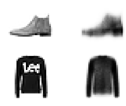
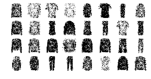
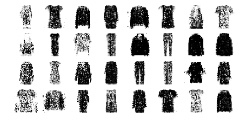
The autoencoder compresses the information so much (down to 16 bits!) that it’s quite lossy, but that’s okay, we’re using it to produce semantic hashes, not to perfectly reconstruct the images:
show_reconstructions(hashing_ae)
plt.show()
Notice that the outputs are indeed very close to 0 or 1 (left graph):
plot_activations_histogram(hashing_encoder)
plt.show()
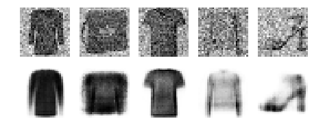
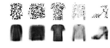
Now let’s see what the hashes look like for the first few images in the validation set:
hashes = np.round(hashing_encoder.predict(X_valid)).astype(np.int32)
hashes *= np.array([[2**bit for bit in range(16)]])
hashes = hashes.sum(axis=1)
for h in hashes[:5]:
    print("{:016b}".format(h))
print("...")
0000100101011011
0000100100110011
0100100100011011
0001100111001010
0001010100110000
...
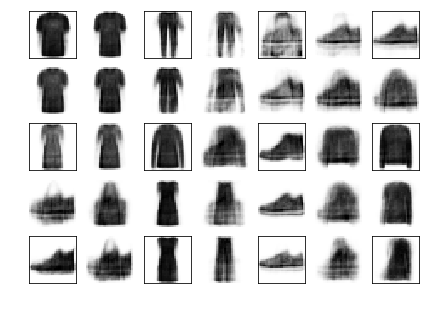
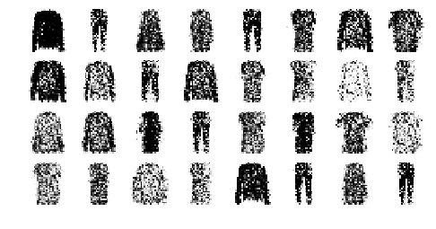
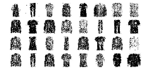
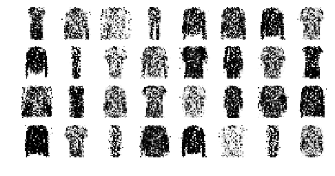
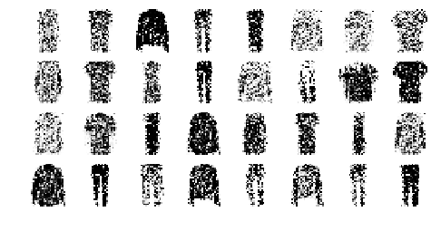
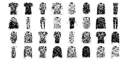
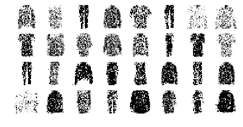
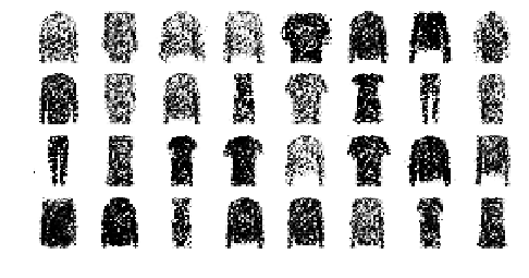
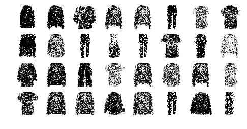
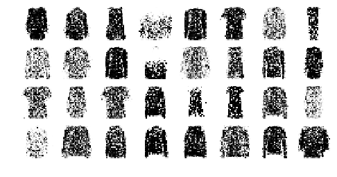
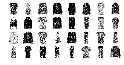
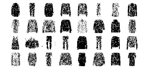
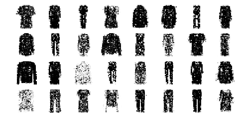
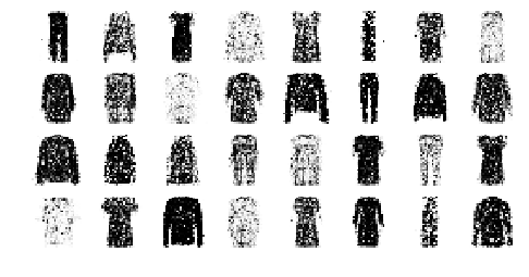
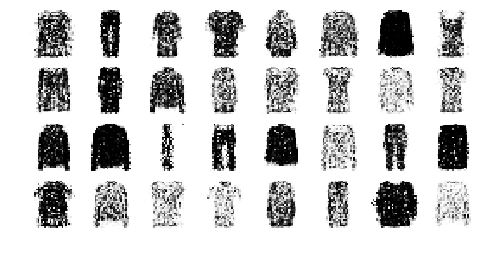
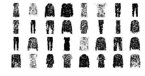
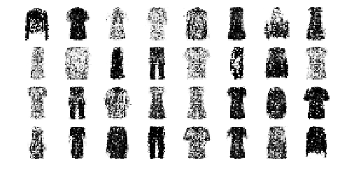
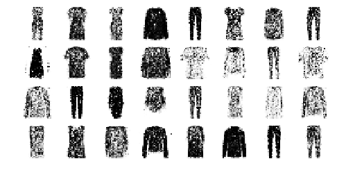
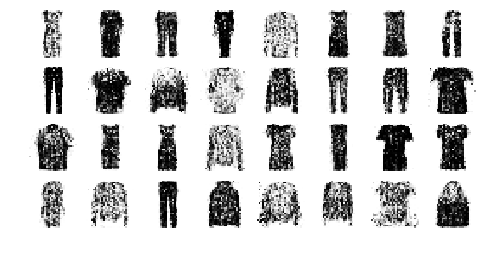
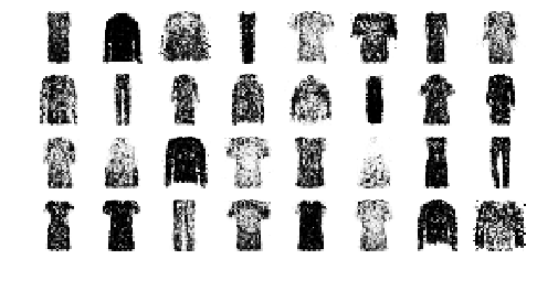
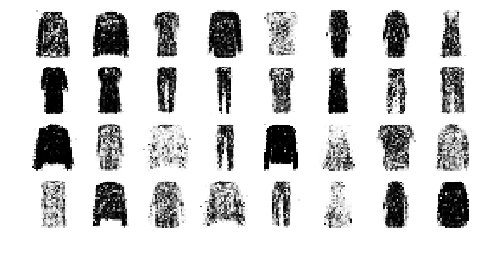
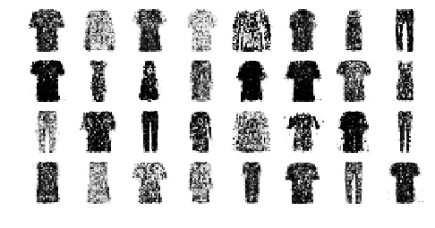
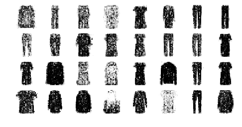
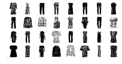
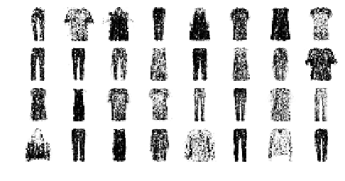
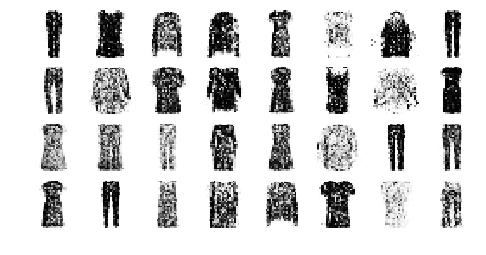
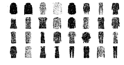
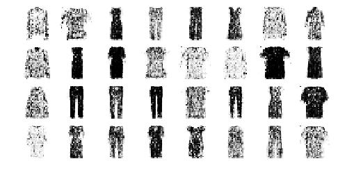
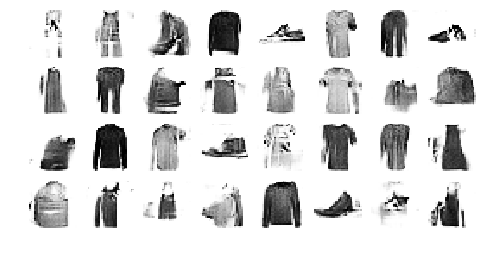
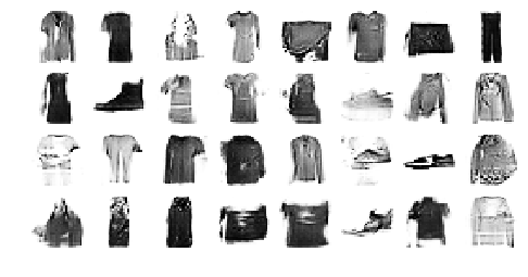
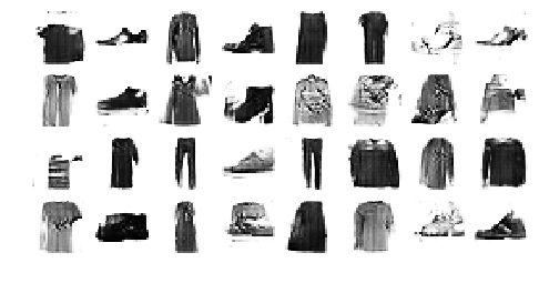
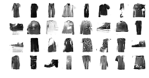
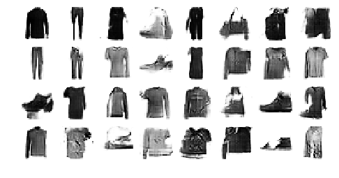
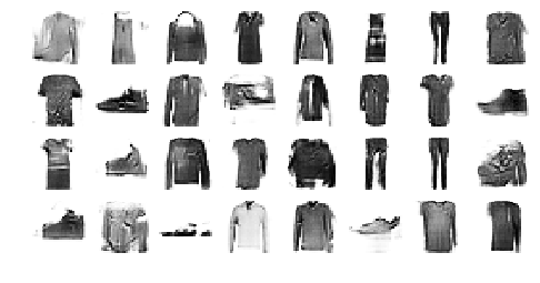
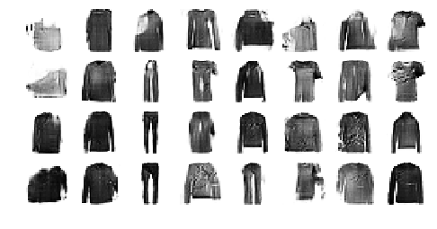
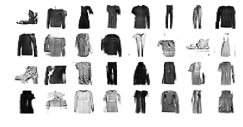
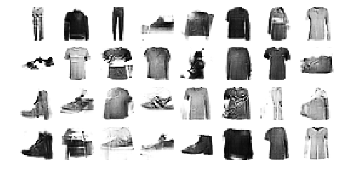
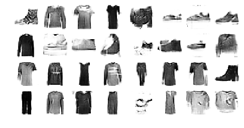
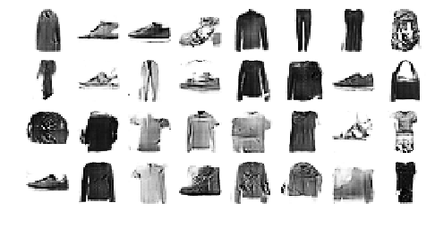
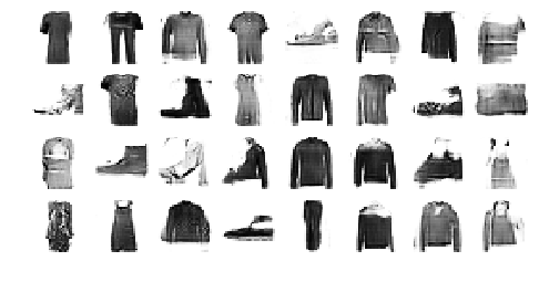
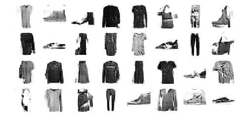
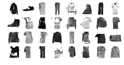
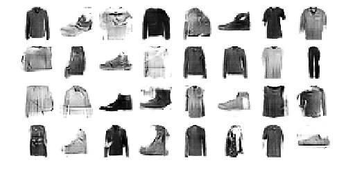
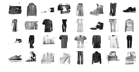
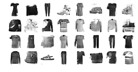
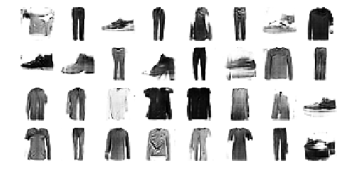
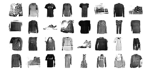
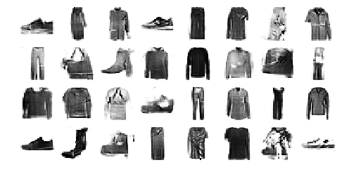
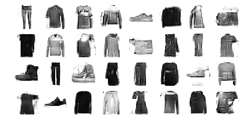
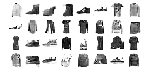
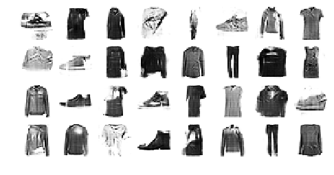
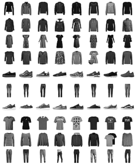
Now let’s find the most common image hashes in the validation set, and display a few images for each hash. In the following image, all the images on a given row have the same hash:
from collections import Counter

n_hashes = 10
n_images = 8

top_hashes = Counter(hashes).most_common(n_hashes)

plt.figure(figsize=(n_images, n_hashes))
for hash_index, (image_hash, hash_count) in enumerate(top_hashes):
    indices = (hashes == image_hash)
    for index, image in enumerate(X_valid[indices][:n_images]):
        plt.subplot(n_hashes, n_images, hash_index * n_images + index + 1)
        plt.imshow(image, cmap="binary")
        plt.axis("off")
Exercise Solutions#
1. to 8.#
See Appendix A.
9.#
Exercise: Try using a denoising autoencoder to pretrain an image classifier. You can use MNIST (the simplest option), or a more complex image dataset such as CIFAR10 if you want a bigger challenge. Regardless of the dataset you’re using, follow these steps:
Split the dataset into a training set and a test set. Train a deep denoising autoencoder on the full training set.
Check that the images are fairly well reconstructed. Visualize the images that most activate each neuron in the coding layer.
Build a classification DNN, reusing the lower layers of the autoencoder. Train it using only 500 images from the training set. Does it perform better with or without pretraining?
[X_train, y_train], [X_test, y_test] = keras.datasets.cifar10.load_data()
X_train = X_train / 255
X_test = X_test / 255
tf.random.set_seed(42)
np.random.seed(42)

denoising_encoder = keras.models.Sequential([
    keras.layers.GaussianNoise(0.1, input_shape=[32, 32, 3]),
    keras.layers.Conv2D(32, kernel_size=3, padding="same", activation="relu"),
    keras.layers.MaxPool2D(),
    keras.layers.Flatten(),
    keras.layers.Dense(512, activation="relu"),
])
denoising_encoder.summary()
Model: "sequential_105"
_________________________________________________________________
Layer (type)                 Output Shape              Param #
=================================================================
gaussian_noise_36 (GaussianN (None, 32, 32, 3)         0
_________________________________________________________________
conv2d_51 (Conv2D)           (None, 32, 32, 32)        896
_________________________________________________________________
max_pooling2d_56 (MaxPooling (None, 16, 16, 32)        0
_________________________________________________________________
flatten_20 (Flatten)         (None, 8192)              0
_________________________________________________________________
dense_70 (Dense)             (None, 512)               4194816
=================================================================
Total params: 4,195,712
Trainable params: 4,195,712
Non-trainable params: 0
_________________________________________________________________
denoising_decoder = keras.models.Sequential([
    keras.layers.Dense(16 * 16 * 32, activation="relu", input_shape=[512]),
    keras.layers.Reshape([16, 16, 32]),
    keras.layers.Conv2DTranspose(filters=3, kernel_size=3, strides=2,
                                 padding="same", activation="sigmoid")
])
denoising_decoder.summary()
Model: "sequential_106"
_________________________________________________________________
Layer (type)                 Output Shape              Param #
=================================================================
dense_71 (Dense)             (None, 8192)              4202496
_________________________________________________________________
reshape_22 (Reshape)         (None, 16, 16, 32)        0
_________________________________________________________________
conv2d_transpose_62 (Conv2DT (None, 32, 32, 3)         867
=================================================================
Total params: 4,203,363
Trainable params: 4,203,363
Non-trainable params: 0
_________________________________________________________________
denoising_ae = keras.models.Sequential([denoising_encoder, denoising_decoder])
denoising_ae.compile(loss="binary_crossentropy", optimizer=keras.optimizers.Nadam(),
                     metrics=["mse"])
history = denoising_ae.fit(X_train, X_train, epochs=10,
                           validation_data=(X_test, X_test))
Train on 50000 samples, validate on 10000 samples
Epoch 1/10
50000/50000 [==============================] - 160s 3ms/sample - loss: 0.5936 - mse: 0.0187 - val_loss: 0.5849 - val_mse: 0.0143
Epoch 2/10
50000/50000 [==============================] - 169s 3ms/sample - loss: 0.5727 - mse: 0.0100 - val_loss: 0.5783 - val_mse: 0.0117
Epoch 3/10
50000/50000 [==============================] - 183s 4ms/sample - loss: 0.5676 - mse: 0.0080 - val_loss: 0.5715 - val_mse: 0.0090
Epoch 4/10
50000/50000 [==============================] - 182s 4ms/sample - loss: 0.5653 - mse: 0.0071 - val_loss: 0.5695 - val_mse: 0.0083
Epoch 5/10
50000/50000 [==============================] - 185s 4ms/sample - loss: 0.5639 - mse: 0.0066 - val_loss: 0.5687 - val_mse: 0.0079
Epoch 6/10
50000/50000 [==============================] - 158s 3ms/sample - loss: 0.5629 - mse: 0.0062 - val_loss: 0.5669 - val_mse: 0.0072
Epoch 7/10
50000/50000 [==============================] - 157s 3ms/sample - loss: 0.5622 - mse: 0.0060 - val_loss: 0.5653 - val_mse: 0.0066
Epoch 8/10
50000/50000 [==============================] - 157s 3ms/sample - loss: 0.5618 - mse: 0.0058 - val_loss: 0.5651 - val_mse: 0.0065
Epoch 9/10
50000/50000 [==============================] - 159s 3ms/sample - loss: 0.5615 - mse: 0.0057 - val_loss: 0.5650 - val_mse: 0.0066
Epoch 10/10
50000/50000 [==============================] - 160s 3ms/sample - loss: 0.5612 - mse: 0.0056 - val_loss: 0.5637 - val_mse: 0.0060
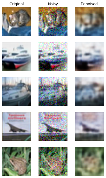
n_images = 5
new_images = X_test[:n_images]
new_images_noisy = new_images + np.random.randn(n_images, 32, 32, 3) * 0.1
new_images_denoised = denoising_ae.predict(new_images_noisy)

plt.figure(figsize=(6, n_images * 2))
for index in range(n_images):
    plt.subplot(n_images, 3, index * 3 + 1)
    plt.imshow(new_images[index])
    plt.axis('off')
    if index == 0:
        plt.title("Original")
    plt.subplot(n_images, 3, index * 3 + 2)
    plt.imshow(np.clip(new_images_noisy[index], 0., 1.))
    plt.axis('off')
    if index == 0:
        plt.title("Noisy")
    plt.subplot(n_images, 3, index * 3 + 3)
    plt.imshow(new_images_denoised[index])
    plt.axis('off')
    if index == 0:
        plt.title("Denoised")
plt.show()
10.#
Exercise: Train a variational autoencoder on the image dataset of your choice, and use it to generate images. Alternatively, you can try to find an unlabeled dataset that you are interested in and see if you can generate new samples.
11.#
Exercise: Train a DCGAN to tackle the image dataset of your choice, and use it to generate images. Add experience replay and see if this helps. Turn it into a conditional GAN where you can control the generated class.